Perform predictive modeling using Machine learning algorithms to inform if a waze user will churn or not.
data science
machine learning
Author
Anshuman Kumar
Published
February 5, 2024
Introduction
The goal of this modeling analysis is to predict whether or not a Waze user is retained or churned. The purpose of this model is to find factors that drive user churn.
This notebook has four stages:
Stage 1: Planning and initial brainstorming Stage 2: Exploratory Data Analysis (EDA) - Perform feature selection, extraction, and transformation to prepare the data for modeling.
Stage 3: Construct Models - Build the models (eg., XGBoost, Random Forest).
Stage 4: Execute - Train Models and Draw Conclusion - Evaluate the models, and propose next steps to stakeholders.
Using PACE framework for problem-solving
We will follow PACE (Plan, Analyze, Construct, Execute) framework to address our goal of predicting user churn. This notebook components are labeled with the respective PACE stage.
Stage 1: Plan
It is essential to commence with planning for the project. Answering the following questions will enable us to gain comprehensive insights and a deeper understanding of the project’s landscape.
Are there any specific technologies or methodologies that need to be used? What are the potential challenges or obstacles that might arise?
Answer
For solving a binary classification problem, we could use a variety of algorithms - Logistic Regression, Support Vector Machine, Decision Trees, Random Forest, Naive Bayes, etc. depending on the specific needs of the project. If we’re dealing with big data, we might consider using Spark, Hadoop, and Kafka. As for methodologies, we’ll likely follow the standard data science process: data collection, data cleaning, exploratory data analysis, model building, and evaluation. There are several challenges that we might encounter. Data quality is a common issue - we need to ensure our data is clean and relevant. Overfitting is another potential problem, where our model performs well on training data but poorly on unseen data. We’ll need to use techniques like cross-validation to mitigate this. We need to check our assumptions. Logistic regression assumes that there is a linear relationship between the logit of the response and the predictors, an assumption that might not hold true for our data. We’ll need to validate this assumption and consider other models if it doesn’t hold.
Who are the key stakeholders involved? What are the expected deliverables? What is the timeline for completion?
Answer
Key stakeholders could include internal teams, external clients, or even regulatory bodies. Knowing who the stakeholders are can help you understand the different perspectives and expectations for the project. You and your team should have a consensus on tangible outputs expected from this project. Once specific details/clarifications are addressed, start with setting a clear timeline with milestones for the project.
How will success of be measured upon completion of the project? What are the consequences of your model making errors? What is the likely effect of the model when it predicts a false negative (i.e., when the model says a Waze user won’t churn, but they actually will)?
Answer
Waze will fail to take proactive measures to retain users who are likely to stop using the app. For example, Waze might proactively push an app notification to users, or send a survey to better understand user dissatisfaction.
What is the likely effect of the model when it predicts a false positive (i.e., when the model says a Waze user will churn, but they actually won’t)
Waze may take proactive measures to retain users who are NOT likely to churn. This may lead to an annoying or negative experience for loyal users of the app.
Do the benefits of such a model outweigh the potential problems?
Answer
The proactive measures taken by Waze might have unintended effects on users, and these effects might encourage user churn. Follow-up analysis on the effectiveness of the measures is recommended. If the measures are reasonable and effective, then the benefits will most likely outweigh the problems.
Would you proceed with the request to build this model? Why or why not? Yes. There aren’t any significant risks for building such a model.
Stage 2: Analyze
2.1: Exploratory Data Analysis
Code
# Import packages for data manipulationimport numpy as npimport pandas as pd# Import packages for data visualizationimport matplotlib.pyplot as plt# This lets us see all of the columns, preventing Juptyer from redacting them.pd.set_option('display.max_columns', None)# Import packages for data modelingfrom sklearn.model_selection import GridSearchCV, train_test_splitfrom sklearn.metrics import roc_auc_score, roc_curve, aucfrom sklearn.metrics import accuracy_score, precision_score, recall_score,\f1_score, confusion_matrix, ConfusionMatrixDisplay, RocCurveDisplay, PrecisionRecallDisplayfrom sklearn.ensemble import RandomForestClassifierfrom xgboost import XGBClassifier# This is the function that helps plot feature importancefrom xgboost import plot_importance# This module lets us save our models once we fit them.import pickle
Building on our data analysis from in previous section, some features had stronger correlations with churn than other. We will also try to creata some features that may be useful. This requires domain knowledge in many situations, and therefore, it is recommeded to have some level of familiarity with such data sets.
In this part, we will engineer these features and some new features to use for modeling.
Create a copy of df0 to preserve the original dataframe. Call the copy df.
Code
# Copy the df0 dataframedf = df0.copy()
Call info() on the new dataframe so the existing columns can be easily referenced.
Create a feature representing the mean number of kilometers driven on each driving day in the last month for each user. Add this feature as a column to df.
count    1.499900e+04
mean              inf
std               NaN
min      3.022063e+00
25%      1.672804e+02
50%      3.231459e+02
75%      7.579257e+02
max               inf
Name: km_per_driving_day, dtype: float64
Notice that some values are infinite. This is the result of there being values of zero in the driving_days column. Pandas imputes a value of infinity in the corresponding rows of the new column because division by zero is undefined.
Code
# 1. Convert infinite values to zerodf.loc[df['km_per_driving_day']==np.inf, 'km_per_driving_day'] =0# 2. Confirm that it workeddf['km_per_driving_day'].describe()
count    14999.000000
mean       578.963113
std       1030.094384
min          0.000000
25%        136.238895
50%        272.889272
75%        558.686918
max      15420.234110
Name: km_per_driving_day, dtype: float64
percent_sessions_in_last_month
Create a new column percent_sessions_in_last_month that represents the percentage of each user’s total sessions that were logged in their last month of use.
count    14999.000000
mean         0.449255
std          0.286919
min          0.000000
25%          0.196221
50%          0.423097
75%          0.687216
max          1.530637
Name: percent_sessions_in_last_month, dtype: float64
professional_driver
Create a new, binary feature called professional_driver that is a 1 for users who had 60 or more drives and drove on 15+ days in the last month.
Note: The objective is to create a new feature that separates professional drivers from other drivers. In this scenario, domain knowledge and intuition are used to determine these deciding thresholds, but ultimately they are arbitrary.
count    14999.000000
mean       190.394608
std        334.674026
min         72.013095
25%         90.706222
50%        122.382022
75%        193.130119
max      23642.920871
Name: km_per_hour, dtype: float64
These numbers are obviously problematic, and it would be worthwhile to seek clarification from Waze regarding how these features are collected to better understand why such unrealistic speeds are observed.
km_per_drive
Create a column representing the mean number of kilometers per drive made in the last month for each user. Then, print descriptive statistics for the feature.
count    1.499900e+04
mean              inf
std               NaN
min      1.008775e+00
25%      3.323065e+01
50%      7.488006e+01
75%      1.854667e+02
max               inf
Name: km_per_drive, dtype: float64
This feature has infinite values too. We will convert the infinite values to zero and then verify that it worked.
Code
# 1. Convert infinite values to zerodf.loc[df['km_per_drive']==np.inf, 'km_per_drive'] =0# 2. Confirm that it workeddf['km_per_drive'].describe()
count    14999.000000
mean       232.817946
std        620.622351
min          0.000000
25%         32.424301
50%         72.854343
75%        179.347527
max      15777.426560
Name: km_per_drive, dtype: float64
percent_of_sessions_to_favorite
Finally, create a new column that represents the percentage of total sessions that were used to navigate to one of the users’ favorite places. Then, print descriptive statistics for the new column.
This is a proxy representation for the percent of overall drives that are to a favorite place. Since total drives since onboarding are not contained in this dataset, total sessions must serve as a reasonable approximation.
People whose drives to non-favorite places make up a higher percentage of their total drives might be less likely to churn, since they’re making more drives to less familiar places.
count    14999.000000
mean         1.665439
std          8.865666
min          0.000000
25%          0.203471
50%          0.649818
75%          1.638526
max        777.563629
Name: percent_of_drives_to_favorite, dtype: float64
2.3: Drop missing values
Because we from previous EDA that there is no evidence of a non-random cause of the 700 missing values in the label column, and because these observations comprise less than 5% of the data, use the dropna() method to drop the rows that are missing this data.
Code
# Drop rows with missing valuesdf = df.dropna(subset=['label'])
2.4: Find outliers
We from previous EDA that many of these columns have outliers. However, tree-based models are resilient to outliers, so there is no need to make any imputations.
2.5: Variable encoding
Dummying features
In order to use device as an X variable, you will need to convert it to binary, since this variable is categorical.
Code
# Create new `device2` variabledf['device2'] = np.where(df['device']=='Android', 0, 1)df[['device', 'device2']].tail()
device
device2
14994
iPhone
1
14995
Android
0
14996
iPhone
1
14997
iPhone
1
14998
iPhone
1
Target encoding
The target variable is also categorical, since a user is labeled as either “churned” or “retained.” Change the data type of the label column to be binary. This change is needed to train the models.
Assign a 0 for all retained users.
Assign a 1 for all churned users.
Save this variable as label2 so as not to overwrite the original label variable.
Approximately 18% of the users in this dataset churned. This is an unbalanced dataset, but not extremely so. It can be modeled without any class rebalancing.
Now, consider which evaluation metric is best. Remember, accuracy might not be the best gauge of performance because a model can have high accuracy on an imbalanced dataset and still fail to predict the minority class.
It was already determined that the risks involved in making a false positive prediction are minimal. No one stands to get hurt, lose money, or suffer any other significant consequence if they are predicted to churn. Therefore, select the model based on the recall score.
3.3: Modeling workflow and model selection process
The final modeling dataset contains 14,299 samples. This is towards the lower end of what might be considered sufficient to conduct a robust model selection process, but still doable.
Split the data into train/validation/test sets (60/20/20)
Note that, when deciding the split ratio and whether or not to use a validation set to select a champion model, consider both how many samples will be in each data partition, and how many examples of the minority class each would therefore contain. In this case, a 60/20/20 split would result in ~2,860 samples in the validation set and the same number in the test set, of which ~18%—or 515 samples—would represent users who churn.
Fit models and tune hyperparameters on the training set
Perform final model selection on the validation set
Assess the champion model’s performance on the test set
Split the data
Now you’re ready to model. The only remaining step is to split the data into features/target variable and training/validation/test sets.
Define a variable X that isolates the features. Remember not to use device.
Define a variable y that isolates the target variable (label2).
Split the data 80/20 into an interim training set and a test set. Don’t forget to stratify the splits, and set the random state to 42.
Split the interim training set 75/25 into a training set and a validation set, yielding a final ratio of 60/20/20 for training/validation/test sets. Again, don’t forget to stratify the splits and set the random state.
Code
# 1. Isolate X variablesX = df.drop(columns=['label', 'label2', 'device'])# 2. Isolate y variabley = df['label2']# 3. Split into train and test setsX_tr, X_test, y_tr, y_test = train_test_split(X, y, stratify=y, test_size=0.2, random_state=42)# 4. Split into train and validate setsX_train, X_val, y_train, y_val = train_test_split(X_tr, y_tr, stratify=y_tr, test_size=0.25, random_state=42)
Verify the number of samples in the partitioned data.
Code
for x in [X_train, X_val, X_test]:print(len(x))
8579
2860
2860
This aligns with expectations.
3.4: Construct Models
Random forest
Begin with using GridSearchCV to tune a random forest model.
Instantiate the random forest classifier rf and set the random state.
Create a dictionary cv_params of any of the following hyperparameters and their corresponding values to tune. The more you tune, the better your model will fit the data, but the longer it will take.
max_depth
max_features
max_samples
min_samples_leaf
min_samples_split
n_estimators
Define a set scoring of scoring metrics for GridSearch to capture (precision, recall, F1 score, and accuracy).
Instantiate the GridSearchCV object rf_cv. Pass to it as arguments:
estimator=rf
param_grid=cv_params
scoring=scoring
cv: define the number of cross-validation folds you want (cv=_)
refit: indicate which evaluation metric you want to use to select the model (refit=_)
refit should be set to 'recall'.
Note: To save time, this notebook doesn’t use multiple values for each parameter in the grid search, but for production run include a range of values in your search to optimize on the best set of parameters.
Code
# 1. Instantiate the random forest classifierrf = RandomForestClassifier(random_state=42)# 2. Create a dictionary of hyperparameters to tunecv_params = {'max_depth': [None],'max_features': [1.0],'max_samples': [1.0],'min_samples_leaf': [2],'min_samples_split': [2],'n_estimators': [300], }# 3. Define a dictionary of scoring metrics to capturescoring = {'accuracy', 'precision', 'recall', 'f1'}# 4. Instantiate the GridSearchCV objectrf_cv = GridSearchCV(rf, cv_params, scoring=scoring, cv=4, refit='recall')
Now fit the model to the training data.
Code
%%timerf_cv.fit(X_train, y_train)
CPU times: user 2min 3s, sys: 57.7 ms, total: 2min 3s
Wall time: 2min 3s
In a Jupyter environment, please rerun this cell to show the HTML representation or trust the notebook. On GitHub, the HTML representation is unable to render, please try loading this page with nbviewer.org.
Use the make_results() function to output all of the scores of your model. Note that the function accepts three arguments.
Code
def make_results(model_name:str, model_object, metric:str):''' Arguments: model_name (string): what you want the model to be called in the output table model_object: a fit GridSearchCV object metric (string): precision, recall, f1, or accuracy Returns a pandas df with the F1, recall, precision, and accuracy scores for the model with the best mean 'metric' score across all validation folds. '''# Create dictionary that maps input metric to actual metric name in GridSearchCV metric_dict = {'precision': 'mean_test_precision','recall': 'mean_test_recall','f1': 'mean_test_f1','accuracy': 'mean_test_accuracy', }# Get all the results from the CV and put them in a df cv_results = pd.DataFrame(model_object.cv_results_)# Isolate the row of the df with the max(metric) score best_estimator_results = cv_results.iloc[cv_results[metric_dict[metric]].idxmax(), :]# Extract accuracy, precision, recall, and f1 score from that row f1 = best_estimator_results.mean_test_f1 recall = best_estimator_results.mean_test_recall precision = best_estimator_results.mean_test_precision accuracy = best_estimator_results.mean_test_accuracy# Create table of results table = pd.DataFrame({'model': [model_name],'precision': [precision],'recall': [recall],'F1': [f1],'accuracy': [accuracy], }, )return table
Pass the GridSearch object to the make_results() function.
Asside from the accuracy, the scores aren’t that good. However, recall that when you built the logistic regression model in the last course the recall was ~0.09, which means that this model has 33% better recall and about the same accuracy, and it was trained on less data.
If you want, feel free to try retuning your hyperparameters to try to get a better score. You might be able to marginally improve the model.
XGBoost
Try to improve your scores using an XGBoost model.
Instantiate the XGBoost classifier xgb and set objective='binary:logistic'. Also set the random state.
Create a dictionary cv_params of the following hyperparameters and their corresponding values to tune:
max_depth
min_child_weight
learning_rate
n_estimators
Define a set scoring of scoring metrics for grid search to capture (precision, recall, F1 score, and accuracy).
Instantiate the GridSearchCV object xgb_cv. Pass to it as arguments:
estimator=xgb
param_grid=cv_params
scoring=scoring
cv: define the number of cross-validation folds you want (cv=_)
refit: indicate which evaluation metric you want to use to select the model (refit='recall')
Code
# 1. Instantiate the XGBoost classifierxgb = XGBClassifier(objective='binary:logistic', random_state=42)# 2. Create a dictionary of hyperparameters to tunecv_params = {'max_depth': [6, 12],'min_child_weight': [3, 5],'learning_rate': [0.01, 0.1],'n_estimators': [300] }# 3. Define a dictionary of scoring metrics to capturescoring = {'accuracy', 'precision', 'recall', 'f1'}# 4. Instantiate the GridSearchCV objectxgb_cv = GridSearchCV(xgb, cv_params, scoring=scoring, cv=4, refit='recall')
Now fit the model to the X_train and y_train data.
Note this cell might take several minutes to run.
Code
%%timexgb_cv.fit(X_train, y_train)
CPU times: user 4min 26s, sys: 1.9 s, total: 4min 28s
Wall time: 2min 16s
In a Jupyter environment, please rerun this cell to show the HTML representation or trust the notebook. On GitHub, the HTML representation is unable to render, please try loading this page with nbviewer.org.
Use the make_results() function to output all of the scores of your model.
Code
# Call 'make_results()' on the GridSearch objectxgb_cv_results = make_results('XGB cv', xgb_cv, 'recall')results = pd.concat([results, xgb_cv_results], axis=0)results
model
precision
recall
F1
accuracy
0
RF cv
0.457163
0.126782
0.198445
0.81851
0
XGB cv
0.442586
0.173468
0.248972
0.81478
This model fit the data even better than the random forest model. The recall score is nearly double the recall score from the logistic regression model from the previous course, and it’s almost 50% better than the random forest model’s recall score, while maintaining a similar accuracy and precision score.
Stage 4: Execute
4.1: Model selection
Now, use the best random forest model and the best XGBoost model to predict on the validation data. Whichever performs better will be selected as the champion model.
Random forest
Code
# Use random forest model to predict on validation datarf_val_preds = rf_cv.best_estimator_.predict(X_val)
Use the get_test_scores() function to generate a table of scores from the predictions on the validation data.
Code
def get_test_scores(model_name:str, preds, y_test_data):''' Generate a table of test scores. In: model_name (string): Your choice: how the model will be named in the output table preds: numpy array of test predictions y_test_data: numpy array of y_test data Out: table: a pandas df of precision, recall, f1, and accuracy scores for your model ''' accuracy = accuracy_score(y_test_data, preds) precision = precision_score(y_test_data, preds) recall = recall_score(y_test_data, preds) f1 = f1_score(y_test_data, preds) table = pd.DataFrame({'model': [model_name],'precision': [precision],'recall': [recall],'F1': [f1],'accuracy': [accuracy] })return table
Code
# Get validation scores for RF modelrf_val_scores = get_test_scores('RF val', rf_val_preds, y_val)# Append to the results tableresults = pd.concat([results, rf_val_scores], axis=0)results
model
precision
recall
F1
accuracy
0
RF cv
0.457163
0.126782
0.198445
0.818510
0
XGB cv
0.442586
0.173468
0.248972
0.814780
0
RF val
0.445255
0.120316
0.189441
0.817483
Notice that the scores went down from the training scores across all metrics, but only by very little. This means that the model did not overfit the training data.
XGBoost
Now, do the same thing to get the performance scores of the XGBoost model on the validation data.
Code
# Use XGBoost model to predict on validation dataxgb_val_preds = xgb_cv.best_estimator_.predict(X_val)# Get validation scores for XGBoost modelxgb_val_scores = get_test_scores('XGB val', xgb_val_preds, y_val)# Append to the results tableresults = pd.concat([results, xgb_val_scores], axis=0)results
model
precision
recall
F1
accuracy
0
RF cv
0.457163
0.126782
0.198445
0.818510
0
XGB cv
0.442586
0.173468
0.248972
0.814780
0
RF val
0.445255
0.120316
0.189441
0.817483
0
XGB val
0.430769
0.165680
0.239316
0.813287
Just like with the random forest model, the XGBoost model’s validation scores were lower, but only very slightly. It is still the clear champion.
4.2: Use champion model to predict on test data
Now, use the champion model to predict on the test dataset. This is to give a final indication of how you should expect the model to perform on new future data, should you decide to use the model.
Code
# Use XGBoost model to predict on test dataxgb_test_preds = xgb_cv.best_estimator_.predict(X_test)# Get test scores for XGBoost modelxgb_test_scores = get_test_scores('XGB test', xgb_test_preds, y_test)# Append to the results tableresults = pd.concat([results, xgb_test_scores], axis=0)results
model
precision
recall
F1
accuracy
0
RF cv
0.457163
0.126782
0.198445
0.818510
0
XGB cv
0.442586
0.173468
0.248972
0.814780
0
RF val
0.445255
0.120316
0.189441
0.817483
0
XGB val
0.430769
0.165680
0.239316
0.813287
0
XGB test
0.388889
0.165680
0.232365
0.805944
The recall was exactly the same as it was on the validation data, but the precision declined notably, which caused all of the other scores to drop slightly. Nonetheless, this is stil within the acceptable range for performance discrepancy between validation and test scores.
4.3: Confusion matrix
Plot a confusion matrix of the champion model’s predictions on the test data.
Code
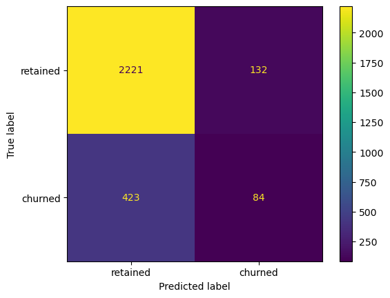
# Generate array of values for confusion matrixcm = confusion_matrix(y_test, xgb_test_preds, labels=xgb_cv.classes_)# Plot confusion matrixdisp = ConfusionMatrixDisplay(confusion_matrix=cm, display_labels=['retained', 'churned'])disp.plot();
The model predicted three times as many false negatives than it did false positives, and it correctly identified only 16.6% of the users who actually churned.
4.4: Feature importance
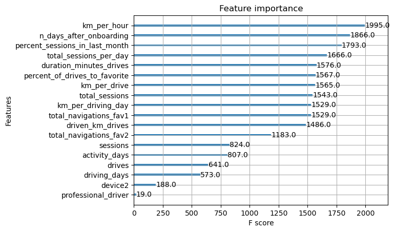
Use the plot_importance function to inspect the most important features of your final model.
Code
plot_importance(xgb_cv.best_estimator_);
The XGBoost model made more use of many of the features than did the logistic regression model, which weighted a single feature (activity_days) very heavily in its final prediction.
If anything, this underscores the importance of feature engineering. Notice that engineered features accounted for six of the top 10 features (and three of the top five). Feature engineering is often one of the best and easiest ways to boost model performance.
Also, note that the important features in one model might not be the same as the important features in another model. That’s why you shouldn’t discount features as unimportant without thoroughly examining them and understanding their relationship with the dependent variable, if possible. These discrepancies between features selected by models are typically caused by complex feature interactions.
Remember, sometimes your data simply will not be predictive of your chosen target. This is common. Machine learning is a powerful tool, but it is not magic. If your data does not contain predictive signal, even the most complex algorithm will not be able to deliver consistent and accurate predictions. Do not be afraid to draw this conclusion.
Even if you cannot use the model to make strong predictions, was the work done in vain? What insights can you report back to stakeholders?
Conclusion
Consider the following questions and think about key points you may want to share with the team, and what information is most relevant to the user churn project.
Questions:
Would you recommend using this model for churn prediction? Why or why not?
Answer
It depends. What would the model be used for? If it’s used to drive consequential business decisions, then no. The model is not a strong enough predictor, as made clear by its poor recall score. However, if the model is only being used to guide further exploratory efforts, then it can have value.
What tradeoff was made by splitting the data into training, validation, and test sets as opposed to just training and test sets?
Answer
Splitting the data three ways means that there is less data available to train the model than splitting just two ways. However, performing model selection on a separate validation set enables testing of the champion model by itself on the test set, which gives a better estimate of future performance than splitting the data two ways and selecting a champion model by performance on the test data.
What is the benefit of using a logistic regression model over an ensemble of tree-based models (like random forest or XGBoost) for classification tasks?
Answer
Logistic regression models are easier to interpret. Because they assign coefficients to predictor variables, they reveal not only which features factored most heavily into their final predictions, but also the directionality of the weight. In other words, they tell you if each feature is positively or negatively correlated with the target in the model’s final prediction.
What is the benefit of using an ensemble of tree-based models like random forest or XGBoost over a logistic regression model for classification tasks?
Answer
Tree-based model ensembles are often better predictors. If the most important thing is the predictive power of the model, then tree-based modeling will usually win out against logistic regression (but not always!). They also require much less data cleaning and require fewer assumptions about the underlying distributions of their predictor variables, so they’re easier to work with.
What could you do to improve this model?
Answer
New features could be engineered to try to generate better predictive signal, as they often do if you have domain knowledge. In the case of this model, the engineered features made up over half of the top 10 most-predictive features used by the model. It could also be helpful to reconstruct the model with different combinations of predictor variables to reduce noise from unpredictive features.
What additional features would you like to have to help improve the model?
Answer
It would be helpful to have drive-level information for each user (such as drive times, geographic locations, etc.). It would probably also be helpful to have more granular data to know how users interact with the app. For example, how often do they report or confirm road hazard alerts? Finally, it could be helpful to know the monthly count of unique starting and ending locations each driver inputs.
Appendix
The following content demonstrates further steps that you might take to tailor your model to your use case.
Identify an optimal decision threshold
The default decision threshold for most implementations of classification algorithms—including scikit-learn’s—is 0.5. This means that, in the case of the Waze models, if they predicted that a given user had a 50% probability or greater of churning, then that user was assigned a predicted value of 1—the user was predicted to churn.
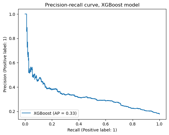
With imbalanced datasets where the response class is a minority, this threshold might not be ideal. You learned that a precision-recall curve can help to visualize the trade-off between your model’s precision and recall.
Here’s the precision-recall curve for the XGBoost champion model on the test data.
As recall increases, precision decreases. But what if you determined that false positives aren’t much of a problem? For example, in the case of this Waze project, a false positive could just mean that a user who will not actually churn gets an email and a banner notification on their phone. It’s very low risk.
So, what if instead of using the default 0.5 decision threshold of the model, you used a lower threshold?
Here’s an example where the threshold is set to 0.4:
Code
# Get predicted probabilities on the test datapredicted_probabilities = xgb_cv.best_estimator_.predict_proba(X_test)predicted_probabilities
The predict_proba() method returns a 2-D array of probabilities where each row represents a user. The first number in the row is the probability of belonging to the negative class, the second number in the row is the probability of belonging to the positive class. (Notice that the two numbers in each row are complimentary to each other and sum to one.)
You can generate new predictions based on this array of probabilities by changing the decision threshold for what is considered a positive response. For example, the following code converts the predicted probabilities to {0, 1} predictions with a threshold of 0.4. In other words, any users who have a value ≥ 0.4 in the second column will get assigned a prediction of 1, indicating that they churned.
Code
# Create a list of just the second column values (probability of target)probs = [x[1] for x in predicted_probabilities]# Create an array of new predictions that assigns a 1 to any value >= 0.4new_preds = np.array([1if x >=0.4else0for x in probs])new_preds
array([0, 1, 0, ..., 0, 0, 0])
Code
# Get evaluation metrics for when the threshold is 0.4get_test_scores('XGB, threshold = 0.4', new_preds, y_test)
model
precision
recall
F1
accuracy
0
XGB, threshold = 0.4
0.383333
0.226824
0.285006
0.798252
Compare these numbers with the results from earlier.
Code
results
model
precision
recall
F1
accuracy
0
RF cv
0.457163
0.126782
0.198445
0.818510
0
XGB cv
0.442586
0.173468
0.248972
0.814780
0
RF val
0.445255
0.120316
0.189441
0.817483
0
XGB val
0.430769
0.165680
0.239316
0.813287
0
XGB test
0.388889
0.165680
0.232365
0.805944
Recall and F1 score increased significantly, while precision and accuracy decreased marginally.
So, using the precision-recall curve as a guide, suppose you knew that you’d be satisfied if the model had a recall score of 0.5 and you were willing to accept the ~30% precision score that comes with it. In other words, you’d be happy if the model successfully identified half of the people who will actually churn, even if it means that when the model says someone will churn, it’s only correct about 30% of the time.
What threshold will yield this result? There are a number of ways to determine this. Here’s one way that uses a function to accomplish this.
Code
def threshold_finder(y_test_data, probabilities, desired_recall):''' Find the decision threshold that most closely yields a desired recall score. Inputs: y_test_data: Array of true y values probabilities: The results of the `predict_proba()` model method desired_recall: The recall that you want the model to have Outputs: threshold: The decision threshold that most closely yields the desired recall recall: The exact recall score associated with `threshold` ''' probs = [x[1] for x in probabilities] # Isolate second column of `probabilities` thresholds = np.arange(0, 1, 0.001) # Set a grid of 1,000 thresholds to test scores = []for threshold in thresholds:# Create a new array of {0, 1} predictions based on new threshold preds = np.array([1if x >= threshold else0for x in probs])# Calculate recall score for that threshold recall = recall_score(y_test_data, preds)# Append the threshold and its corresponding recall score as a tuple to `scores` scores.append((threshold, recall)) distances = []for idx, score inenumerate(scores):# Calculate how close each actual score is to the desired score distance =abs(score[1] - desired_recall)# Append the (index#, distance) tuple to `distances` distances.append((idx, distance))# Sort `distances` by the second value in each of its tuples (least to greatest) sorted_distances =sorted(distances, key=lambda x: x[1], reverse=False)# Identify the tuple with the actual recall closest to desired recall best = sorted_distances[0]# Isolate the index of the threshold with the closest recall score best_idx = best[0]# Retrieve the threshold and actual recall score closest to desired recall threshold, recall = scores[best_idx]return threshold, recall
Now, test the function to find the threshold that results in a recall score closest to 0.5.
Code
# Get the predicted probabilities from the champion modelprobabilities = xgb_cv.best_estimator_.predict_proba(X_test)# Call the functionthreshold_finder(y_test, probabilities, 0.5)
(0.124, 0.5029585798816568)
Setting a threshold of 0.124 will result in a recall of 0.503.
To verify, you can repeat the steps performed earlier to get the other evaluation metrics for when the model has a threshold of 0.124. Based on the precision-recall curve, a 0.5 recall score should have a precision of ~0.3.
Code
# Create an array of new predictions that assigns a 1 to any value >= 0.124probs = [x[1] for x in probabilities]new_preds = np.array([1if x >=0.124else0for x in probs])# Get evaluation metrics for when the threshold is 0.124get_test_scores('XGB, threshold = 0.124', new_preds, y_test)
model
precision
recall
F1
accuracy
0
XGB, threshold = 0.124
0.304296
0.502959
0.379182
0.708042
It worked! Hopefully we now understand that changing the decision threshold is another tool that can help achieve useful results from the model.