In this notebook, you will learn about Neural Style Transfer, an algorithm created by Gatys et al. (2015).
Upon completion of this assignment, you will be able to: - Implement the neural style transfer algorithm - Generate novel artistic images using your algorithm - Define the style cost function for Neural Style Transfer - Define the content cost function for Neural Style Transfer
Most of the algorithms you’ve studied optimize a cost function to get a set of parameter values. With Neural Style Transfer, you’ll get to optimize a cost function to get pixel values. Exciting!|
Packages
Run the following code cell to import the necessary packages and dependencies you will need to perform Neural Style Transfer.
Code
import osimport sysimport scipy.ioimport scipy.miscimport matplotlib.pyplot as pltfrom matplotlib.pyplot import imshowfrom PIL import Imageimport numpy as npimport tensorflow as tfimport pprintfrom public_tests import*%matplotlib inline
Problem Statement
Neural Style Transfer (NST) is one of the most fun and interesting optimization techniques in deep learning. It merges two images, namely: a “content” image (C) and a “style” image (S), to create a “generated” image (G). The generated image G combines the “content” of the image C with the “style” of image S.
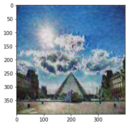
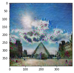
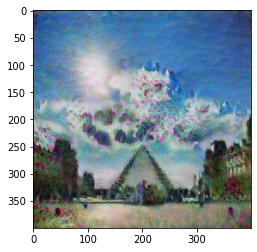
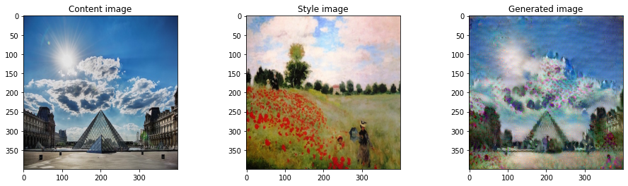
In this assignment, you are going to combine the Louvre museum in Paris (content image C) with the impressionist style of Claude Monet (style image S) to generate the following image:
Transfer Learning
Neural Style Transfer (NST) uses a previously trained convolutional network, and builds on top of that. The idea of using a network trained on a different task and applying it to a new task is called transfer learning.
You will be using the eponymously named VGG network from the original NST paper published by the Visual Geometry Group at University of Oxford in 2014. Specifically, you’ll use VGG-19, a 19-layer version of the VGG network. This model has already been trained on the very large ImageNet database, and has learned to recognize a variety of low level features (at the shallower layers) and high level features (at the deeper layers).
Run the following code to load parameters from the VGG model. This may take a few seconds.
Code
tf.random.set_seed(272) # DO NOT CHANGE THIS VALUEpp = pprint.PrettyPrinter(indent=4)img_size =400vgg = tf.keras.applications.VGG19(include_top=False, input_shape=(img_size, img_size, 3), weights='pretrained-model/vgg19_weights_tf_dim_ordering_tf_kernels_notop.h5')vgg.trainable =Falsepp.pprint(vgg)
<keras.engine.functional.Functional object at 0x7f6c70238f70>
Neural Style Transfer (NST)
Next, you will be building the Neural Style Transfer (NST) algorithm in three steps:
First, you will build the content cost function \(J_{content}(C,G)\)
Second, you will build the style cost function \(J_{style}(S,G)\)
Finally, you’ll put it all together to get \(J(G) = \alpha J_{content}(C,G) + \beta J_{style}(S,G)\). Exciting!
Computing the Content Cost
Make Generated Image G Match the Content of Image C
One goal you should aim for when performing NST is for the content in generated image G to match the content of image C. To do so, you’ll need an understanding of shallow versus deep layers :
The shallower layers of a ConvNet tend to detect lower-level features such as edges and simple textures.
The deeper layers tend to detect higher-level features such as more complex textures and object classes.
To choose a “middle” activation layer \(a^{[l]}\) :
You need the “generated” image G to have similar content as the input image C. Suppose you have chosen some layer’s activations to represent the content of an image. * In practice, you will usually get the most visually pleasing results if you choose a layer from somewhere in the middle of the network–neither too shallow nor too deep. This ensures that the network detects both higher-level and lower-level features. * After you have finished this exercise, feel free to come back and experiment with using different layers to see how the results vary!
To forward propagate image “C:”
Set the image C as the input to the pretrained VGG network, and run forward propagation.
Let \(a^{(C)}\) be the hidden layer activations in the layer you had chosen. (In lecture, this was written as \(a^{[l](C)}\), but here the superscript \([l]\) is dropped to simplify the notation.) This will be an \(n_H \times n_W \times n_C\) tensor.
To forward propagate image “G”:
Repeat this process with the image G: Set G as the input, and run forward propagation.
Let \(a^{(G)}\) be the corresponding hidden layer activation.
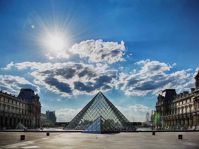
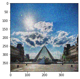
In this running example, the content image C will be the picture of the Louvre Museum in Paris. Run the code below to see a picture of the Louvre.
Code
content_image = Image.open("images/louvre.jpg")print("The content image (C) shows the Louvre museum's pyramid surrounded by old Paris buildings, against a sunny sky with a few clouds.")content_image
The content image (C) shows the Louvre museum's pyramid surrounded by old Paris buildings, against a sunny sky with a few clouds.
Content Cost Function \(J_{content}(C,G)\)
One goal you should aim for when performing NST is for the content in generated image G to match the content of image C. A method to achieve this is to calculate the content cost function, which will be defined as:
Here, \(n_H, n_W\) and \(n_C\) are the height, width and number of channels of the hidden layer you have chosen, and appear in a normalization term in the cost.
For clarity, note that \(a^{(C)}\) and \(a^{(G)}\) are the 3D volumes corresponding to a hidden layer’s activations.
In order to compute the cost \(J_{content}(C,G)\), it might also be convenient to unroll these 3D volumes into a 2D matrix, as shown below.
Technically this unrolling step isn’t needed to compute \(J_{content}\), but it will be good practice for when you do need to carry out a similar operation later for computing the style cost \(J_{style}\).
compute_content_cost
Compute the “content cost” using TensorFlow.
Instructions:
a_G: hidden layer activations representing content of the image G a_C: hidden layer activations representing content of the image C
The 3 steps to implement this function are: 1. Retrieve dimensions from a_G: - To retrieve dimensions from a tensor X, use: X.get_shape().as_list() 2. Unroll a_C and a_G as explained in the picture above - You’ll likely want to use these functions: tf.transpose and tf.reshape. 3. Compute the content cost: - You’ll likely want to use these functions: tf.reduce_sum, tf.square and tf.subtract.
Additional Hints for “Unrolling”
To unroll the tensor, you want the shape to change from \((m,n_H,n_W,n_C)\) to \((m, n_H \times n_W, n_C)\).
tf.reshape(tensor, shape) takes a list of integers that represent the desired output shape.
For the shape parameter, a -1 tells the function to choose the correct dimension size so that the output tensor still contains all the values of the original tensor.
So tf.reshape(a_C, shape=[m, n_H * n_W, n_C]) gives the same result as tf.reshape(a_C, shape=[m, -1, n_C]).
If you prefer to re-order the dimensions, you can use tf.transpose(tensor, perm), where perm is a list of integers containing the original index of the dimensions.
For example, tf.transpose(a_C, perm=[0,3,1,2]) changes the dimensions from \((m, n_H, n_W, n_C)\) to \((m, n_C, n_H, n_W)\).
Again, note that you don’t necessarily need tf.transpose to ‘unroll’ the tensors in this case but this is a useful function to practice and understand for other situations that you’ll encounter.
Code
def compute_content_cost(content_output, generated_output):""" Computes the content cost Arguments: a_C -- tensor of dimension (1, n_H, n_W, n_C), hidden layer activations representing content of the image C a_G -- tensor of dimension (1, n_H, n_W, n_C), hidden layer activations representing content of the image G Returns: J_content -- scalar that you compute using equation 1 above. """ a_C = content_output[-1] a_G = generated_output[-1]# Retrieve dimensions from a_G (≈1 line) _, n_H, n_W, n_C = a_G.get_shape().as_list()# Reshape 'a_C' and 'a_G' (≈2 lines)# DO NOT reshape 'content_output' or 'generated_output' a_C_unrolled = tf.reshape(a_C, shape=[_, n_H * n_W, n_C]) a_G_unrolled = tf.reshape(a_G, shape=[_, n_H * n_W, n_C])# compute the cost with tensorflow (≈1 line) J_content = tf.reduce_sum(tf.square(a_C_unrolled - a_G_unrolled))/(4.0* n_H * n_W * n_C)return J_content
Code
### you cannot edit this cellcompute_content_cost_test(compute_content_cost)
J_content = tf.Tensor(7.056877, shape=(), dtype=float32)
All tests passed
You’ve now successfully calculated the content cost function!
What you should remember:
The content cost takes a hidden layer activation of the neural network, and measures how different \(a^{(C)}\) and \(a^{(G)}\) are.
When you minimize the content cost later, this will help make sure \(G\) has similar content as \(C\).
Computing the Style Cost
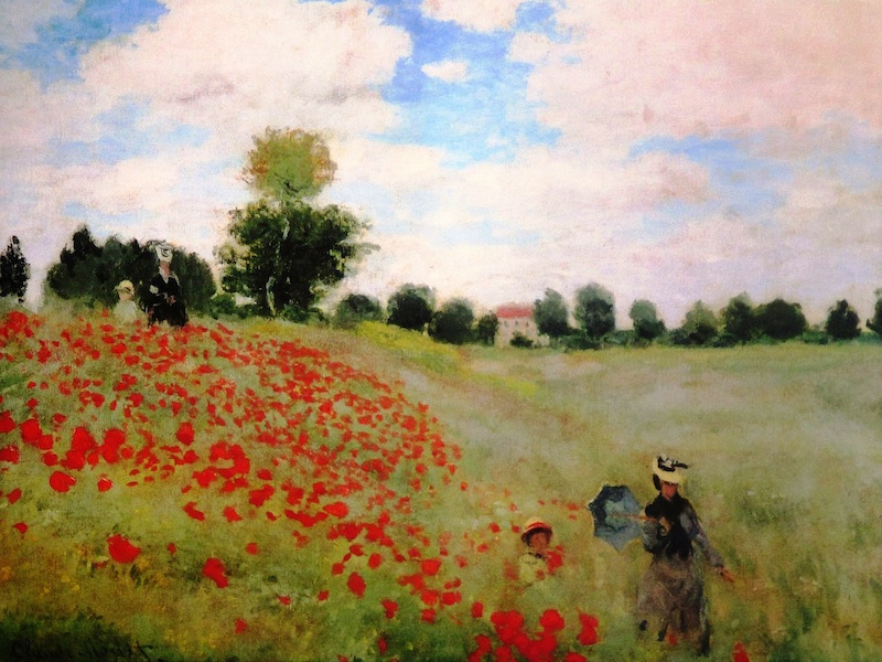
For the running example, you will use the following style image:
Code
example = Image.open("images/monet_800600.jpg")example
Now let’s see how you can now define a “style” cost function \(J_{style}(S,G)\)!
Style Matrix
Gram matrix
The style matrix is also called a “Gram matrix.”
In linear algebra, the Gram matrix G of a set of vectors \((v_{1},\dots ,v_{n})\) is the matrix of dot products, whose entries are \({\displaystyle G_{ij} = v_{i}^T v_{j} = np.dot(v_{i}, v_{j}) }\).
In other words, \(G_{ij}\) compares how similar \(v_i\) is to \(v_j\): If they are highly similar, you would expect them to have a large dot product, and thus for \(G_{ij}\) to be large.
Two meanings of the variable \(G\)
Note that there is an unfortunate collision in the variable names used here. Following the common terminology used in the literature:
\(G\) is used to denote the Style matrix (or Gram matrix)
\(G\) also denotes the generated image.
For the sake of clarity, in this assignment \(G_{gram}\) will be used to refer to the Gram matrix, and \(G\) to denote the generated image.
Compute Gram matrix \(G_{gram}\)
You will compute the Style matrix by multiplying the “unrolled” filter matrix with its transpose:
The result is a matrix of dimension \((n_C,n_C)\) where \(n_C\) is the number of filters (channels). The value \(G_{(gram)i,j}\) measures how similar the activations of filter \(i\) are to the activations of filter \(j\).
\(G_{(gram),ii}\): prevalence of patterns or textures
The diagonal elements \(G_{(gram)ii}\) measure how “active” a filter \(i\) is.
For example, suppose filter \(i\) is detecting vertical textures in the image. Then \(G_{(gram)ii}\) measures how common vertical textures are in the image as a whole.
If \(G_{(gram)ii}\) is large, this means that the image has a lot of vertical texture.
By capturing the prevalence of different types of features (\(G_{(gram)ii}\)), as well as how much different features occur together (\(G_{(gram)ij}\)), the Style matrix \(G_{gram}\) measures the style of an image.
gram_matrix
Using TensorFlow, implement a function that computes the Gram matrix of a matrix A.
The formula is: The gram matrix of A is \(G_A = AA^T\).
def gram_matrix(A):""" Argument: A -- matrix of shape (n_C, n_H*n_W) Returns: GA -- Gram matrix of A, of shape (n_C, n_C) """ GA = tf.matmul(A, tf.transpose(A))return GA
Code
### you cannot edit this cellgram_matrix_test(gram_matrix)
You now know how to calculate the Gram matrix. Congrats! Your next goal will be to minimize the distance between the Gram matrix of the “style” image S and the Gram matrix of the “generated” image G. * For now, you will use only a single hidden layer \(a^{[l]}\).
* The corresponding style cost for this layer is defined as:
\(G_{gram}^{(S)}\) Gram matrix of the “style” image.
\(G_{gram}^{(G)}\) Gram matrix of the “generated” image.
Make sure you remember that this cost is computed using the hidden layer activations for a particular hidden layer in the network \(a^{[l]}\)
compute_layer_style_cost
Compute the style cost for a single layer.
Instructions: The 3 steps to implement this function are: 1. Retrieve dimensions from the hidden layer activations a_G: - To retrieve dimensions from a tensor X, use: X.get_shape().as_list() 2. Unroll the hidden layer activations a_S and a_G into 2D matrices, as explained in the picture above (see the images in the sections “computing the content cost” and “style matrix”). - You may use tf.transpose and tf.reshape. 3. Compute the Style matrix of the images S and G. (Use the function you had previously written.) 4. Compute the Style cost: - You may find tf.reduce_sum, tf.square and tf.subtract useful.
Additional Hints
Since the activation dimensions are \((m, n_H, n_W, n_C)\) whereas the desired unrolled matrix shape is \((n_C, n_H*n_W)\), the order of the filter dimension \(n_C\) is changed. So tf.transpose can be used to change the order of the filter dimension.
Code
def compute_layer_style_cost(a_S, a_G):""" Arguments: a_S -- tensor of dimension (1, n_H, n_W, n_C), hidden layer activations representing style of the image S a_G -- tensor of dimension (1, n_H, n_W, n_C), hidden layer activations representing style of the image G Returns: J_style_layer -- tensor representing a scalar value, style cost defined above by equation (2) """# Retrieve dimensions from a_G (≈1 line) _, n_H, n_W, n_C = a_G.get_shape().as_list()# Reshape the tensors from (1, n_H, n_W, n_C) to (n_C, n_H * n_W) (≈2 lines) a_S = tf.transpose(tf.reshape(a_S, shape=[-1, n_C])) a_G = tf.transpose(tf.reshape(a_G, shape=[-1, n_C]))# Computing gram_matrices for both images S and G (≈2 lines) GS = gram_matrix(a_S) GG = gram_matrix(a_G)# Computing the loss (≈1 line) J_style_layer = tf.reduce_sum(tf.square(GS - GG))/(4.0*(( n_H * n_W * n_C)**2))return J_style_layer
Code
### you cannot edit this cellcompute_layer_style_cost_test(compute_layer_style_cost)
J_style_layer = tf.Tensor(14.01649, shape=(), dtype=float32)
All tests passed
Style Weights
So far you have captured the style from only one layer.
You’ll get better results if you “merge” style costs from several different layers.
Each layer will be given weights (\(\lambda^{[l]}\)) that reflect how much each layer will contribute to the style.
After completing this exercise, feel free to come back and experiment with different weights to see how it changes the generated image \(G\).
By default, give each layer equal weight, and the weights add up to 1. (\(\sum_{l}^L\lambda^{[l]} = 1\))
where the values for \(\lambda^{[l]}\) are given in STYLE_LAYERS.
compute_style_cost
Instructions: * A compute_style_cost(…) function has already been implemented. * It calls your compute_layer_style_cost(...) several times, and weights their results using the values in STYLE_LAYERS. * Please read over it to make sure you understand what it’s doing.
Description of compute_style_cost
For each layer: * Select the activation (the output tensor) of the current layer. * Get the style of the style image “S” from the current layer. * Get the style of the generated image “G” from the current layer. * Compute the “style cost” for the current layer * Add the weighted style cost to the overall style cost (J_style)
Once you’re done with the loop:
* Return the overall style cost.
Code
### you cannot edit this celldef compute_style_cost(style_image_output, generated_image_output, STYLE_LAYERS=STYLE_LAYERS):""" Computes the overall style cost from several chosen layers Arguments: style_image_output -- our tensorflow model generated_image_output -- STYLE_LAYERS -- A python list containing: - the names of the layers we would like to extract style from - a coefficient for each of them Returns: J_style -- tensor representing a scalar value, style cost defined above by equation (2) """# initialize the overall style cost J_style =0# Set a_S to be the hidden layer activation from the layer we have selected.# The last element of the array contains the content layer image, which must not be used. a_S = style_image_output[:-1]# Set a_G to be the output of the choosen hidden layers.# The last element of the list contains the content layer image which must not be used. a_G = generated_image_output[:-1]for i, weight inzip(range(len(a_S)), STYLE_LAYERS): # Compute style_cost for the current layer J_style_layer = compute_layer_style_cost(a_S[i], a_G[i])# Add weight * J_style_layer of this layer to overall style cost J_style += weight[1] * J_style_layerreturn J_style
How do you choose the coefficients for each layer? The deeper layers capture higher-level concepts, and the features in the deeper layers are less localized in the image relative to each other. So if you want the generated image to softly follow the style image, try choosing larger weights for deeper layers and smaller weights for the first layers. In contrast, if you want the generated image to strongly follow the style image, try choosing smaller weights for deeper layers and larger weights for the first layers.
What you should remember:
The style of an image can be represented using the Gram matrix of a hidden layer’s activations.
You get even better results by combining this representation from multiple different layers.
This is in contrast to the content representation, where usually using just a single hidden layer is sufficient.
Minimizing the style cost will cause the image \(G\) to follow the style of the image \(S\).
Defining the Total Cost to Optimize
Finally, you will create a cost function that minimizes both the style and the content cost. The formula is:
Implement the total cost function which includes both the content cost and the style cost.
Code
@tf.function()def total_cost(J_content, J_style, alpha =10, beta =40):""" Computes the total cost function Arguments: J_content -- content cost coded above J_style -- style cost coded above alpha -- hyperparameter weighting the importance of the content cost beta -- hyperparameter weighting the importance of the style cost Returns: J -- total cost as defined by the formula above. """ J = alpha*J_content + beta*J_stylereturn J
Code
### you cannot edit this celltotal_cost_test(total_cost)
J = tf.Tensor(32.9832, shape=(), dtype=float32)
All tests passed
What you should remember: - The total cost is a linear combination of the content cost \(J_{content}(C,G)\) and the style cost \(J_{style}(S,G)\). - \(\alpha\) and \(\beta\) are hyperparameters that control the relative weighting between content and style.
Solving the Optimization Problem
Finally, you get to put everything together to implement Neural Style Transfer!
Here’s what your program be able to do:
Load the content image
Load the style image
Randomly initialize the image to be generated
Load the VGG19 model
Compute the content cost
Compute the style cost
Compute the total cost
Define the optimizer and learning rate
Here are the individual steps in detail.
Load the Content Image
Run the following code cell to load, reshape, and normalize your “content” image C (the Louvre museum picture):
Now, you get to initialize the “generated” image as a noisy image created from the content_image.
The generated image is slightly correlated with the content image.
By initializing the pixels of the generated image to be mostly noise but slightly correlated with the content image, this will help the content of the “generated” image more rapidly match the content of the “content” image.
Next, as explained in part(2), define a function which loads the VGG19 model and returns a list of the outputs for the middle layers.
Code
def get_layer_outputs(vgg, layer_names):""" Creates a vgg model that returns a list of intermediate output values.""" outputs = [vgg.get_layer(layer[0]).output for layer in layer_names] model = tf.keras.Model([vgg.input], outputs)return model
Now, define the content layer and build the model.
You’ve built the model, and now to compute the content cost, you will encode your content image using the appropriate hidden layer activations. Set this encoding to the variable a_C. Later in the assignment, you will need to do the same for the generated image, by setting the variable a_G to be the appropriate hidden layer activations. You will use layer block5_conv4 to compute the encoding. The code below does the following:
Set a_C to be the tensor giving the hidden layer activation for layer “block5_conv4” using the content image.
Code
# Assign the content image to be the input of the VGG model. # Set a_C to be the hidden layer activation from the layer we have selectedpreprocessed_content = tf.Variable(tf.image.convert_image_dtype(content_image, tf.float32))a_C = vgg_model_outputs(preprocessed_content)
Compute the Style image Encoding (a_S)
The code below sets a_S to be the tensor giving the hidden layer activation for STYLE_LAYERS using our style image.
Code
# Assign the input of the model to be the "style" image preprocessed_style = tf.Variable(tf.image.convert_image_dtype(style_image, tf.float32))a_S = vgg_model_outputs(preprocessed_style)
Below are the utils that you will need to display the images generated by the style transfer model.
Code
def clip_0_1(image):""" Truncate all the pixels in the tensor to be between 0 and 1 Arguments: image -- Tensor J_style -- style cost coded above Returns: Tensor """return tf.clip_by_value(image, clip_value_min=0.0, clip_value_max=1.0)def tensor_to_image(tensor):""" Converts the given tensor into a PIL image Arguments: tensor -- Tensor Returns: Image: A PIL image """ tensor = tensor *255 tensor = np.array(tensor, dtype=np.uint8)if np.ndim(tensor) >3:assert tensor.shape[0] ==1 tensor = tensor[0]return Image.fromarray(tensor)
train_step
Implement the train_step() function for transfer learning
Use the Adam optimizer to minimize the total cost J.
Compute the encoding of the generated image using vgg_model_outputs. Assign the result to a_G.
Compute the total cost J, using the global variables a_C, a_S and the local a_G
Use alpha = 10 and beta = 40.
Code
optimizer = tf.keras.optimizers.Adam(learning_rate=0.01)@tf.function()def train_step(generated_image):with tf.GradientTape() as tape:# In this function you must use the precomputed encoded images a_S and a_C# Compute a_G as the vgg_model_outputs for the current generated image a_G = vgg_model_outputs(generated_image)# Compute the style cost J_style = compute_style_cost(a_S, a_G)# Compute the content cost J_content = compute_content_cost(a_C, a_G)# Compute the total cost J = total_cost(J_content, J_style) grad = tape.gradient(J, generated_image) optimizer.apply_gradients([(grad, generated_image)]) generated_image.assign(clip_0_1(generated_image))return J
Code
### you cannot edit this cell# You always must run the last cell before this one. You will get an error if not.generated_image = tf.Variable(generated_image)train_step_test(train_step, generated_image)
tf.Tensor(25700.346, shape=(), dtype=float32)
tf.Tensor(17778.395, shape=(), dtype=float32)
All tests passed
Looks like it’s working! Now you’ll get to put it all together into one function to better see your results!
Train the Model
Run the following cell to generate an artistic image. It should take about 3min on a GPU for 2500 iterations. Neural Style Transfer is generally trained using GPUs.
If you increase the learning rate you can speed up the style transfer, but often at the cost of quality.
Code
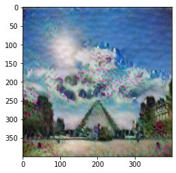
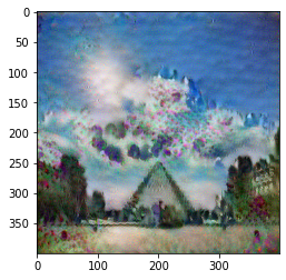
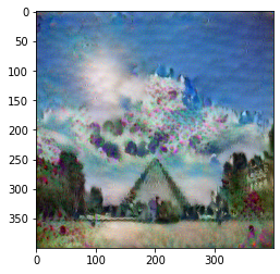
# Show the generated image at some epochs# Uncomment to reset the style transfer process. You will need to compile the train_step function again epochs =2501for i inrange(epochs): train_step(generated_image)if i %250==0:print(f"Epoch {i} ")if i %250==0: image = tensor_to_image(generated_image) imshow(image) image.save(f"output/image_{i}.jpg") plt.show()
Now, run the following code cell to see the results!
Code
# Show the 3 images in a rowfig = plt.figure(figsize=(16, 4))ax = fig.add_subplot(1, 3, 1)imshow(content_image[0])ax.title.set_text('Content image')ax = fig.add_subplot(1, 3, 2)imshow(style_image[0])ax.title.set_text('Style image')ax = fig.add_subplot(1, 3, 3)imshow(generated_image[0])ax.title.set_text('Generated image')plt.show()
Look at that! You did it! After running this, in the upper bar of the notebook click on “File” and then “Open”. Go to the “/output” directory to see all the saved images. Open “generated_image” to see the generated image! :)
Running for around 20000 epochs with a learning rate of 0.001, you should see something like the image presented below on the right:
The hyperparameters were set so that you didn’t have to wait too long to see an initial result. To get the best looking results, you may want to try running the optimization algorithm longer (and perhaps with a smaller learning rate). After completing and submitting this assignment, come back and play more with this notebook, and see if you can generate even better looking images.
Conclusion
You are now able to use Neural Style Transfer to generate artistic images. This is also your first time building a model in which the optimization algorithm updates the pixel values rather than the neural network’s parameters. Deep learning has many different types of models and this is only one of them!
What you should remember
Neural Style Transfer is an algorithm that given a content image C and a style image S can generate an artistic image
It uses representations (hidden layer activations) based on a pretrained ConvNet.
The content cost function is computed using one hidden layer’s activations.
The style cost function for one layer is computed using the Gram matrix of that layer’s activations. The overall style cost function is obtained using several hidden layers.
Optimizing the total cost function results in synthesizing new images.
References
The Neural Style Transfer algorithm was due to Gatys et al. (2015). Harish Narayanan and Github user “log0” also have highly readable write-ups this lab was inspired by. The pre-trained network used in this implementation is a VGG network, which is due to Simonyan and Zisserman (2015). Pre-trained weights were from the work of the MathConvNet team.