In this notebook, we will implement convolutional (CONV) and pooling (POOL) layers in numpy, including both forward propagation and backward propagation.
By the end of this notebook, you’ll be able to:
Explain the convolution operation
Apply two different types of pooling operation
Identify the components used in a convolutional neural network (padding, stride, filter, …) and their purpose
Build a convolutional neural network
Notation: - Superscript \([l]\) denotes an object of the \(l^{th}\) layer. - Example: \(a^{[4]}\) is the \(4^{th}\) layer activation. \(W^{[5]}\) and \(b^{[5]}\) are the \(5^{th}\) layer parameters.
Superscript \((i)\) denotes an object from the \(i^{th}\) example.
Example: \(x^{(i)}\) is the \(i^{th}\) training example input.
Subscript \(i\) denotes the \(i^{th}\) entry of a vector.
Example: \(a^{[l]}_i\) denotes the \(i^{th}\) entry of the activations in layer \(l\), assuming this is a fully connected (FC) layer.
\(n_H\), \(n_W\) and \(n_C\) denote respectively the height, width and number of channels of a given layer. If you want to reference a specific layer \(l\), you can also write \(n_H^{[l]}\), \(n_W^{[l]}\), \(n_C^{[l]}\).
\(n_{H_{prev}}\), \(n_{W_{prev}}\) and \(n_{C_{prev}}\) denote respectively the height, width and number of channels of the previous layer. If referencing a specific layer \(l\), this could also be denoted \(n_H^{[l-1]}\), \(n_W^{[l-1]}\), \(n_C^{[l-1]}\).
Packages
Let’s first import all the packages that you will need during this assignment. - numpy is the fundamental package for scientific computing with Python. - matplotlib is a library to plot graphs in Python. - np.random.seed(1) is used to keep all the random function calls consistent. This helps to grade your work.
Code
import numpy as npimport h5pyimport matplotlib.pyplot as pltfrom public_tests import*%matplotlib inlineplt.rcParams['figure.figsize'] = (5.0, 4.0) # set default size of plotsplt.rcParams['image.interpolation'] ='nearest'plt.rcParams['image.cmap'] ='gray'%load_ext autoreload%autoreload 2np.random.seed(1)
Outline
You will be implementing the building blocks of a convolutional neural network! Each function you will implement will have detailed instructions to walk you through the steps:
Convolution functions, including:
Zero Padding
Convolve window
Convolution forward
Convolution backward (optional)
Pooling functions, including:
Pooling forward
Create mask
Distribute value
Pooling backward (optional)
This notebook will implement these functions from scratch in numpy.
Note: For every forward function, there is a corresponding backward equivalent. Hence, at every step of your forward module you will store some parameters in a cache. These parameters are used to compute gradients during backpropagation.
Convolutional Neural Networks
A convolution layer transforms an input volume into an output volume of different size.
In this part, build every step of the convolution layer. You will first implement two helper functions: one for zero padding and the other for computing the convolution function itself.
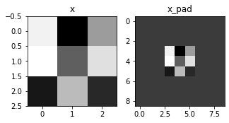
Zero-Padding
Zero-padding adds zeros around the border of an image:
The main benefits of padding are:
It allows you to use a CONV layer without necessarily shrinking the height and width of the volumes. This is important for building deeper networks, since otherwise the height/width would shrink as you go to deeper layers. An important special case is the “same” convolution, in which the height/width is exactly preserved after one layer.
It helps us keep more of the information at the border of an image. Without padding, very few values at the next layer would be affected by pixels at the edges of an image.
zero_pad
Implement the following function, which pads all the images of a batch of examples X with zeros. Use np.pad. Note if you want to pad the array “a” of shape \((5,5,5,5,5)\) with pad = 1 for the 2nd dimension, pad = 3 for the 4th dimension and pad = 0 for the rest, you would do:
In this part, implement a single step of convolution, in which you apply the filter to a single position of the input. This will be used to build a convolutional unit, which:
Takes an input volume
Applies a filter at every position of the input
Outputs another volume (usually of different size)
In a computer vision application, each value in the matrix on the left corresponds to a single pixel value. You convolve a 3x3 filter with the image by multiplying its values element-wise with the original matrix, then summing them up and adding a bias. In this first step of the exercise, you will implement a single step of convolution, corresponding to applying a filter to just one of the positions to get a single real-valued output.
Later in this notebook, you’ll apply this function to multiple positions of the input to implement the full convolutional operation.
Note: The variable b will be passed in as a numpy array. If you add a scalar (a float or integer) to a numpy array, the result is a numpy array. In the special case of a numpy array containing a single value, you can cast it as a float to convert it to a scalar.
Code
def conv_single_step(a_slice_prev, W, b):""" Apply one filter defined by parameters W on a single slice (a_slice_prev) of the output activation of the previous layer. Arguments: a_slice_prev -- slice of input data of shape (f, f, n_C_prev) W -- Weight parameters contained in a window - matrix of shape (f, f, n_C_prev) b -- Bias parameters contained in a window - matrix of shape (1, 1, 1) Returns: Z -- a scalar value, the result of convolving the sliding window (W, b) on a slice x of the input data """ s = np.multiply(a_slice_prev,W)# Sum over all entries of the volume s. Z = np.sum(s)# Add bias b to Z. Cast b to a float() so that Z results in a scalar value. b = np.squeeze(b) Z = Z + b return Z
In the forward pass, you will take many filters and convolve them on the input. Each ‘convolution’ gives you a 2D matrix output. You will then stack these outputs to get a 3D volume:
conv_forward
Implement the function below to convolve the filters W on an input activation A_prev.
This function takes the following inputs: * A_prev, the activations output by the previous layer (for a batch of m inputs); * Weights are denoted by W. The filter window size is f by f. * The bias vector is b, where each filter has its own (single) bias.
You also have access to the hyperparameters dictionary, which contains the stride and the padding.
Hint: 1. To select a 2x2 slice at the upper left corner of a matrix “a_prev” (shape (5,5,3)), you would do:
a_slice_prev = a_prev[0:2,0:2,:]
Notice how this gives a 3D slice that has height 2, width 2, and depth 3. Depth is the number of channels.
This will be useful when you will define a_slice_prev below, using the start/end indexes you will define.
To define a_slice you will need to first define its corners vert_start, vert_end, horiz_start and horiz_end. This figure may be helpful for you to find out how each of the corners can be defined using h, w, f and s in the code below.
Reminder:
The formulas relating the output shape of the convolution to the input shape are:
\[n_H = \Bigl\lfloor \frac{n_{H_{prev}} - f + 2 \times pad}{stride} \Bigr\rfloor +1\]\[n_W = \Bigl\lfloor \frac{n_{W_{prev}} - f + 2 \times pad}{stride} \Bigr\rfloor +1\]\[n_C = \text{number of filters used in the convolution}\]
For this exercise, don’t worry about vectorization! Just implement everything with for-loops.
Additional Hints (if you’re stuck):
Use array slicing (e.g.varname[0:1,:,3:5]) for the following variables: a_prev_pad ,W, b
Copy the starter code of the function and run it outside of the defined function, in separate cells.
Check that the subset of each array is the size and dimension that you’re expecting.
To decide how to get the vert_start, vert_end, horiz_start, horiz_end, remember that these are indices of the previous layer.
Draw an example of a previous padded layer (8 x 8, for instance), and the current (output layer) (2 x 2, for instance).
The output layer’s indices are denoted by h and w.
Make sure that a_slice_prev has a height, width and depth.
Remember that a_prev_pad is a subset of A_prev_pad.
Think about which one should be used within the for loops.
Code
def conv_forward(A_prev, W, b, hparameters):""" Implements the forward propagation for a convolution function Arguments: A_prev -- output activations of the previous layer, numpy array of shape (m, n_H_prev, n_W_prev, n_C_prev) W -- Weights, numpy array of shape (f, f, n_C_prev, n_C) b -- Biases, numpy array of shape (1, 1, 1, n_C) hparameters -- python dictionary containing "stride" and "pad" Returns: Z -- conv output, numpy array of shape (m, n_H, n_W, n_C) cache -- cache of values needed for the conv_backward() function """# Retrieve dimensions from A_prev's shape (≈1 line) (m, n_H_prev, n_W_prev, n_C_prev) = A_prev.shape# Retrieve dimensions from W's shape (≈1 line) (f, f, n_C_prev, n_C) = W.shape# Retrieve information from "hparameters" (≈2 lines) stride = hparameters["stride"] pad = hparameters["pad"]# Compute the dimensions of the CONV output volume using the formula given above. # Hint: use int() to apply the 'floor' operation. (≈2 lines) n_H =int((n_H_prev +2*pad - f)/stride) +1 n_W =int((n_W_prev +2*pad - f)/stride) +1# Initialize the output volume Z with zeros. (≈1 line) Z = np.zeros((m, n_H, n_W, n_C))# Create A_prev_pad by padding A_prev A_prev_pad = zero_pad(A_prev, pad)for i inrange(m): # loop over the batch of training examples a_prev_pad = A_prev_pad[i] # Select ith training example's padded activationfor h inrange(n_H): # loop over vertical axis of the output volume# Find the vertical start and end of the current "slice" (≈2 lines) vert_start = stride * h vert_end = vert_start + ffor w inrange(n_W): # loop over horizontal axis of the output volume# Find the horizontal start and end of the current "slice" (≈2 lines) horiz_start = stride * w horiz_end = horiz_start + ffor c inrange(n_C): # loop over channels (= #filters) of the output volume# Use the corners to define the (3D) slice of a_prev_pad (See Hint above the cell). (≈1 line) a_slice_prev = a_prev_pad[vert_start:vert_end,horiz_start:horiz_end,:]# Convolve the (3D) slice with the correct filter W and bias b, to get back one output neuron. (≈3 line) weights = W[:, :, :, c] biases = b[:, :, :, c] Z[i, h, w, c] = conv_single_step(a_slice_prev, weights, biases)# Save information in "cache" for the backprop cache = (A_prev, W, b, hparameters)return Z, cache
Z's mean =
 0.5511276474566768
Z[0,2,1] =
 [-2.17796037  8.07171329 -0.5772704   3.36286738  4.48113645 -2.89198428
 10.99288867  3.03171932]
cache_conv[0][1][2][3] =
 [-1.1191154   1.9560789  -0.3264995  -1.34267579]
First Test: All tests passed!
Second Test: All tests passed!
Finally, a CONV layer should also contain an activation, in which case you would add the following line of code:
# Convolve the window to get back one output neuronZ[i, h, w, c] = ...# Apply activationA[i, h, w, c] = activation(Z[i, h, w, c])
You don’t need to do it here, however.
Pooling Layer
The pooling (POOL) layer reduces the height and width of the input. It helps reduce computation, as well as helps make feature detectors more invariant to its position in the input. The two types of pooling layers are:
Max-pooling layer: slides an (\(f, f\)) window over the input and stores the max value of the window in the output.
Average-pooling layer: slides an (\(f, f\)) window over the input and stores the average value of the window in the output.
These pooling layers have no parameters for backpropagation to train. However, they have hyperparameters such as the window size \(f\). This specifies the height and width of the \(f \times f\) window you would compute a max or average over.
Forward Pooling
Now, you are going to implement MAX-POOL and AVG-POOL, in the same function.
pool_forward
Implement the forward pass of the pooling layer. Follow the hints in the comments below.
Reminder: As there’s no padding, the formulas binding the output shape of the pooling to the input shape is:
def pool_forward(A_prev, hparameters, mode ="max"):""" Implements the forward pass of the pooling layer Arguments: A_prev -- Input data, numpy array of shape (m, n_H_prev, n_W_prev, n_C_prev) hparameters -- python dictionary containing "f" and "stride" mode -- the pooling mode you would like to use, defined as a string ("max" or "average") Returns: A -- output of the pool layer, a numpy array of shape (m, n_H, n_W, n_C) cache -- cache used in the backward pass of the pooling layer, contains the input and hparameters """# Retrieve dimensions from the input shape (m, n_H_prev, n_W_prev, n_C_prev) = A_prev.shape# Retrieve hyperparameters from "hparameters" f = hparameters["f"] stride = hparameters["stride"]# Define the dimensions of the output n_H =int(1+ (n_H_prev - f) / stride) n_W =int(1+ (n_W_prev - f) / stride) n_C = n_C_prev# Initialize output matrix A A = np.zeros((m, n_H, n_W, n_C)) for i inrange(m): # loop over the training examples a_prev_slice = A_prev[i]for h inrange(n_H): # loop on the vertical axis of the output volume# Find the vertical start and end of the current "slice" (≈2 lines) vert_start = stride * h vert_end = vert_start + ffor w inrange(n_W): # loop on the horizontal axis of the output volume# Find the vertical start and end of the current "slice" (≈2 lines) horiz_start = stride * w horiz_end = horiz_start + ffor c inrange (n_C): # loop over the channels of the output volume# Use the corners to define the current slice on the ith training example of A_prev, channel c. (≈1 line) a_slice_prev = a_prev_slice[vert_start:vert_end,horiz_start:horiz_end,c]# Compute the pooling operation on the slice. # Use an if statement to differentiate the modes. # Use np.max and np.mean.if mode =="max": A[i, h, w, c] = np.max(a_slice_prev)elif mode =="average": A[i, h, w, c] = np.mean(a_slice_prev)else:print(mode+"-type pooling layer NOT Defined") # Store the input and hparameters in "cache" for pool_backward() cache = (A_prev, hparameters)# Making sure your output shape is correctassert(A.shape == (m, n_H, n_W, n_C))return A, cache
A convolution extracts features from an input image by taking the dot product between the input data and a 3D array of weights (the filter).
The 2D output of the convolution is called the feature map
A convolution layer is where the filter slides over the image and computes the dot product
This transforms the input volume into an output volume of different size
Zero padding helps keep more information at the image borders, and is helpful for building deeper networks, because you can build a CONV layer without shrinking the height and width of the volumes
Pooling layers gradually reduce the height and width of the input by sliding a 2D window over each specified region, then summarizing the features in that region
Implemented the forward passes of all the layers of a convolutional network.