Anshuman Kumar - Predicting Amazon next-day stock price direction

Problem Statement

The task is to predict the day price direction of Amazon.com, Inc. (AMZN).

The stock market is very complex and highly volatile. In order to be profitable, we do not need to predict the correct price, but rather, the price direction: whether it will be higher or lower than the price that is today. If we predict it to be higher, we might as well buy some stocks, else, we should probably sell. Therefore, the target would be a binary classification whether the next day closing price will be higher than the opening price.

We have data for the period from 1997 up to the year 2020 that we have split into training (1997-2016), validation (2016-2018) and testing (2018-2020) periods. The data is available in the AMZN_train.csv, AMZN_val.csv and AMZN_test.csv files, respectively.

Data Exploration

Code

import pandas as pd
df_train = pd.read_csv("datasets/AMZN_train.csv")

Code

df_train

	Date	Open	High	Low	Close	Adj Close	Volume
0	1997-05-15	2.437500	2.500000	1.927083	1.958333	1.958333	72156000
1	1997-05-16	1.968750	1.979167	1.708333	1.729167	1.729167	14700000
2	1997-05-19	1.760417	1.770833	1.625000	1.708333	1.708333	6106800
3	1997-05-20	1.729167	1.750000	1.635417	1.635417	1.635417	5467200
4	1997-05-21	1.635417	1.645833	1.375000	1.427083	1.427083	18853200
...	...	...	...	...	...	...	...
4776	2016-05-09	673.950012	686.979980	671.409973	679.750000	679.750000	3982200
4777	2016-05-10	694.000000	704.549988	693.500000	703.070007	703.070007	6105600
4778	2016-05-11	705.789978	719.000000	701.650024	713.229980	713.229980	7338200
4779	2016-05-12	717.380005	722.450012	711.510010	717.929993	717.929993	5048200
4780	2016-05-13	714.640015	719.250000	706.510010	709.919983	709.919983	4763400

4781 rows × 7 columns

Code

df_train.shape

(4781, 7)

Code

df_train.info()

<class 'pandas.core.frame.DataFrame'>
RangeIndex: 4781 entries, 0 to 4780
Data columns (total 7 columns):
 #   Column     Non-Null Count  Dtype  
---  ------     --------------  -----  
 0   Date       4781 non-null   object 
 1   Open       4781 non-null   float64
 2   High       4781 non-null   float64
 3   Low        4781 non-null   float64
 4   Close      4781 non-null   float64
 5   Adj Close  4781 non-null   float64
 6   Volume     4781 non-null   int64  
dtypes: float64(5), int64(1), object(1)
memory usage: 261.6+ KB

Code

df_train.describe()

	Open	High	Low	Close	Adj Close	Volume
count	4781.000000	4781.000000	4781.000000	4781.000000	4781.000000	4.781000e+03
mean	127.619845	129.480122	125.697925	127.662449	127.662449	8.225935e+06
std	145.693083	147.132537	144.053633	145.677581	145.677581	7.810188e+06
min	1.406250	1.447917	1.312500	1.395833	1.395833	4.872000e+05
25%	34.299999	34.849998	33.660000	34.310001	34.310001	4.200900e+06
50%	62.880001	64.750000	60.937500	62.750000	62.750000	6.200100e+06
75%	189.009995	191.600006	186.210007	189.029999	189.029999	9.239900e+06
max	717.380005	722.450012	711.510010	717.929993	717.929993	1.043292e+08

Code

df_train["Date"].describe()

count           4781
unique          4781
top       1997-05-15
freq               1
Name: Date, dtype: object

Code

df_train["Date"].min(), df_train["Date"].max()

('1997-05-15', '2016-05-13')

Code

from matplotlib import pyplot as plt

plt.rcParams["figure.figsize"] = (12, 9)

Code

_ = df_train.plot(x="Date", y=["Close", "Open", "High", "Low"])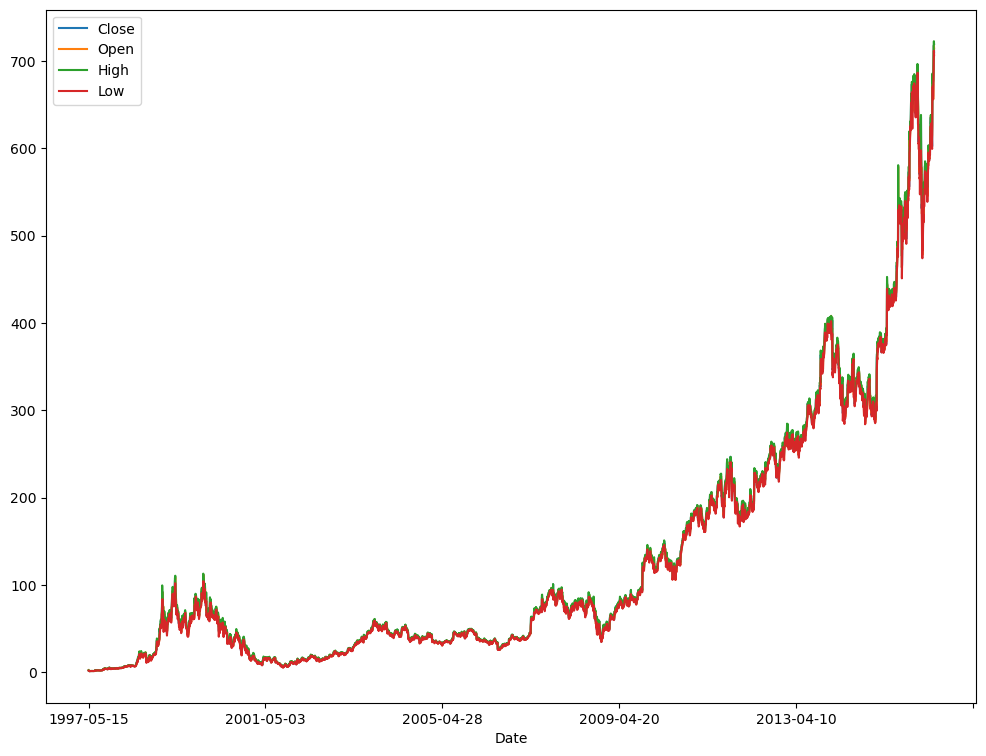

We would like to repeat the same analysis for the validation and testing set, to make sure that they follow a similar distribution and that there are no surprising errors there. We create a function to do that.

Code

def analyse(dataframe):
    """Runs an exploration analysis of the dataframe."""
    print("Shape", dataframe.shape, "\n")
    print("Columns", dataframe.columns, "\n")
    dataframe.info()
    print("\n", dataframe.describe(), "\n")
    print("The data ranges from", dataframe["Date"].min(), "to", dataframe["Date"].max())
    dataframe.plot(x="Date", y=["Close", "Open", "High", "Low"])

Code

# read validation and test sets and then analyse them
df_val = pd.read_csv("datasets/AMZN_val.csv")
analyse(df_val)

Shape (503, 7) 

Columns Index(['Date', 'Open', 'High', 'Low', 'Close', 'Adj Close', 'Volume'], dtype='object') 

<class 'pandas.core.frame.DataFrame'>
RangeIndex: 503 entries, 0 to 502
Data columns (total 7 columns):
 #   Column     Non-Null Count  Dtype  
---  ------     --------------  -----  
 0   Date       503 non-null    object 
 1   Open       503 non-null    float64
 2   High       503 non-null    float64
 3   Low        503 non-null    float64
 4   Close      503 non-null    float64
 5   Adj Close  503 non-null    float64
 6   Volume     503 non-null    int64  
dtypes: float64(5), int64(1), object(1)
memory usage: 27.6+ KB

               Open         High          Low        Close    Adj Close  \
count   503.000000   503.000000   503.000000   503.000000   503.000000   
mean    992.201292   999.898131   982.574513   991.828966   991.828966   
std     255.496588   259.220381   250.100614   254.885469   254.885469   
min     689.559998   696.820007   682.119995   691.359985   691.359985   
25%     780.500000   785.625000   772.410004   780.294983   780.294983   
50%     948.000000   954.400024   941.140015   948.229980   948.229980   
75%    1125.349976  1131.750000  1120.369995  1126.500000  1126.500000   
max    1634.010010  1638.099976  1603.439941  1609.079956  1609.079956   

             Volume  
count  5.030000e+02  
mean   3.918924e+06  
std    2.069197e+06  
min    1.458800e+06  
25%    2.655050e+06  
50%    3.324800e+06  
75%    4.469000e+06  
max    1.656500e+07   

The data ranges from 2016-05-16 to 2018-05-14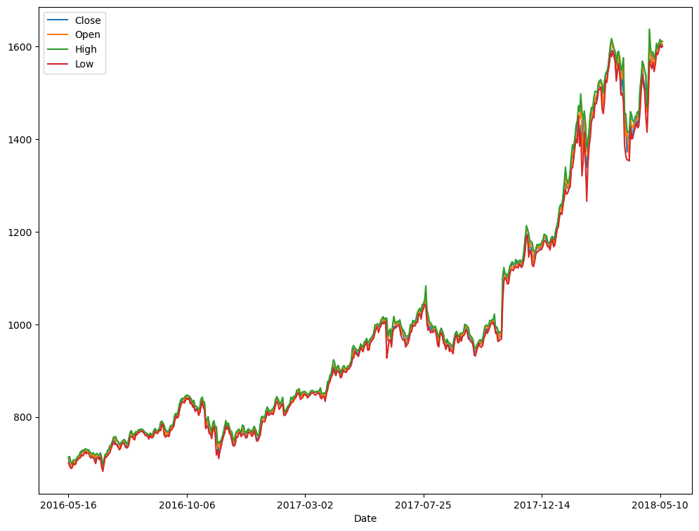

Code

df_test = pd.read_csv("datasets/AMZN_test.csv")
analyse(df_test)

Shape (504, 7) 

Columns Index(['Date', 'Open', 'High', 'Low', 'Close', 'Adj Close', 'Volume'], dtype='object') 

<class 'pandas.core.frame.DataFrame'>
RangeIndex: 504 entries, 0 to 503
Data columns (total 7 columns):
 #   Column     Non-Null Count  Dtype  
---  ------     --------------  -----  
 0   Date       504 non-null    object 
 1   Open       504 non-null    float64
 2   High       504 non-null    float64
 3   Low        504 non-null    float64
 4   Close      504 non-null    float64
 5   Adj Close  504 non-null    float64
 6   Volume     504 non-null    int64  
dtypes: float64(5), int64(1), object(1)
memory usage: 27.7+ KB

               Open         High          Low        Close    Adj Close  \
count   504.000000   504.000000   504.000000   504.000000   504.000000   
mean   1823.927758  1843.069246  1803.067065  1824.040536  1824.040536   
std     178.129809   179.294163   177.457741   178.470078   178.470078   
min    1346.000000  1396.030029  1307.000000  1343.959961  1343.959961   
25%    1712.924988  1730.602447  1691.637543  1713.642517  1713.642517   
50%    1806.539978  1824.244995  1791.289978  1806.119995  1806.119995   
75%    1908.154968  1921.580048  1887.580017  1902.842468  1902.842468   
max    2443.199951  2475.000000  2396.010010  2474.000000  2474.000000   

             Volume  
count  5.040000e+02  
mean   4.705042e+06  
std    2.288185e+06  
min    8.813000e+05  
25%    3.078725e+06  
50%    4.068450e+06  
75%    5.763300e+06  
max    1.556730e+07   

The data ranges from 2018-05-15 to 2020-05-14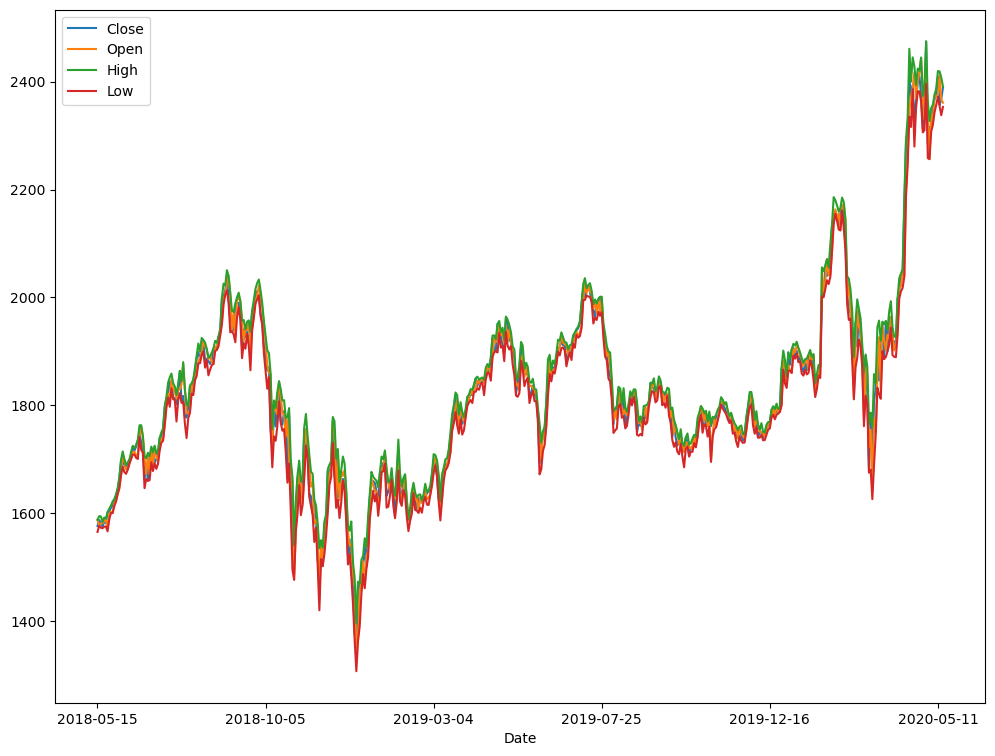

Once we have done our exploration of the data, we can move on to the predictive modeling part of the task. The task was to predict if the next day’s closing price will be higher than the opening price. We do not have that information explicitly in our data, so we have to infer it.

This is relatively simple, we just need to compare the closing and opening prices one day in advance.

To achieve that, first, we will make sure that the data is sorted by the date. We can use the sort_values method and pass in the Date column as a parameter, sorting it in ascending order.

Next, we need to shift the DataFrame by one row / one day and compare the prices. Pandas has a method for doing exactly that, the shift method. We specify a period of minus one (so that we shift the data from the next day back). Because it is a logical operation, Pandas would return a True / False result for each comparison. We want this to be presented as 1 / 0 for the machine learning models, so we will map it to type int. To store all of this information, we will create a new column, called Target.

Code

df_train.sort_values(by="Date", inplace=True)
df_val.sort_values(by="Date", inplace=True)
df_test.sort_values(by="Date", inplace=True)

Code

# notice that we shift by a period of '-1', this takes the next day's price direction for the current day
# a positive period will take the days from the past
df_train["Target"] = (df_train["Close"] > df_train["Open"]).shift(periods=-1, fill_value=0).astype(int)

Code

df_train

	Date	Open	High	Low	Close	Adj Close	Volume	Target
0	1997-05-15	2.437500	2.500000	1.927083	1.958333	1.958333	72156000	0
1	1997-05-16	1.968750	1.979167	1.708333	1.729167	1.729167	14700000	0
2	1997-05-19	1.760417	1.770833	1.625000	1.708333	1.708333	6106800	0
3	1997-05-20	1.729167	1.750000	1.635417	1.635417	1.635417	5467200	0
4	1997-05-21	1.635417	1.645833	1.375000	1.427083	1.427083	18853200	0
...	...	...	...	...	...	...	...	...
4776	2016-05-09	673.950012	686.979980	671.409973	679.750000	679.750000	3982200	1
4777	2016-05-10	694.000000	704.549988	693.500000	703.070007	703.070007	6105600	1
4778	2016-05-11	705.789978	719.000000	701.650024	713.229980	713.229980	7338200	1
4779	2016-05-12	717.380005	722.450012	711.510010	717.929993	717.929993	5048200	0
4780	2016-05-13	714.640015	719.250000	706.510010	709.919983	709.919983	4763400	0

4781 rows × 8 columns

Code

df_train["Target"].value_counts()

Target
1    2392
0    2389
Name: count, dtype: int64

Code

df_val["Target"] = (df_val["Close"] > df_val["Open"]).shift(periods=-1, fill_value=0).astype(int)
df_val["Target"].value_counts()

Target
0    255
1    248
Name: count, dtype: int64

Code

df_test["Target"] = (df_test["Close"] > df_test["Open"]).shift(periods=-1, fill_value=0).astype(int)
df_test["Target"].value_counts()

Target
1    255
0    249
Name: count, dtype: int64

Feature Engineering

Code

df_train["Moving_Average_3"] = (df_train["Close"] - df_train["Open"]).rolling(window=3, min_periods=1).mean()
df_val["Moving_Average_3"] = (df_val["Close"] - df_val["Open"]).rolling(window=3, min_periods=1).mean()
df_test["Moving_Average_3"] = (df_test["Close"] - df_test["Open"]).rolling(window=3, min_periods=1).mean()

Code

df_train["Moving_Average_7"] = (df_train["Close"] - df_train["Open"]).rolling(window=7, min_periods=1).mean()
df_val["Moving_Average_7"] = (df_val["Close"] - df_val["Open"]).rolling(window=7, min_periods=1).mean()
df_test["Moving_Average_7"] = (df_test["Close"] - df_test["Open"]).rolling(window=7, min_periods=1).mean()

Code

# current price direction
df_train["Today_Direction"] = df_train["Close"] - df_train["Open"]
df_val["Today_Direction"] = df_val["Close"] - df_val["Open"]
df_test["Today_Direction"] = df_test["Close"] - df_test["Open"]

Code

# price range
df_train["Price_Range"] = df_train["High"] - df_train["Low"]
df_val["Price_Range"] = df_val["High"] - df_val["Low"]
df_test["Price_Range"] = df_test["High"] - df_test["Low"]

Code

df_train.sample(10, random_state=42)

	Date	Open	High	Low	Close	Adj Close	Volume	Target	Moving_Average_3	Moving_Average_7	Today_Direction	Price_Range
2895	2008-11-14	43.610001	44.500000	41.500000	41.750000	41.750000	11949700	0	-0.253335	-0.601429	-1.860001	3.000000
4430	2014-12-22	301.940002	307.359985	301.940002	306.540009	306.540009	4003800	0	0.436666	-0.705710	4.600007	5.419983
3618	2011-09-29	234.169998	234.300003	216.289993	222.440002	222.440002	9378500	0	-6.126663	-2.434283	-11.729996	18.010010
763	2000-05-24	46.437500	49.750000	40.437500	48.562500	48.562500	11666600	0	-0.937500	-0.580357	2.125000	9.312500
4392	2014-10-28	289.760010	298.000000	289.760010	295.589996	295.589996	5572600	0	4.253326	2.681423	5.829986	8.239990
4657	2015-11-16	640.919983	649.989990	622.289978	647.809998	647.809998	7435900	0	-7.243347	-0.264299	6.890015	27.700012
4008	2013-04-22	259.350006	264.600006	258.029999	263.549988	263.549988	2119100	1	-0.343333	-0.287140	4.199982	6.570007
555	1999-07-29	51.187500	52.187500	50.000000	50.781250	50.781250	18748000	0	-0.841146	-0.713170	-0.406250	2.187500
2754	2008-04-28	80.639999	82.500000	80.120003	81.970001	81.970001	10991900	0	1.453336	1.212857	1.330002	2.379997
33	1997-07-02	1.515625	1.593750	1.510417	1.588542	1.588542	3882000	1	0.026042	0.004464	0.072917	0.083333

Machine Learning Algorithms

Code

# this is the target column that we aim to predict
y_col = "Target"
# these are the input features for the models
X_cols = [
    "Open",
    "Close",
    "High",
    "Low",
    "Volume",
    "Adj Close",
    "Today_Direction",
    "Price_Range",
    "Moving_Average_3",
    "Moving_Average_7"
]

Code

X_train = df_train[X_cols]
y_train = df_train[y_col]

X_val = df_val[X_cols]
y_val = df_val[y_col]

X_test = df_val[X_cols]
y_test = df_val[y_col]

Logistic Regression

Code

# for reproducibility
RANDOM_SEED = 42

Code

from sklearn.linear_model import LogisticRegression
from sklearn.preprocessing import StandardScaler
from sklearn.metrics import  RocCurveDisplay

# use default parameters
lr = LogisticRegression()

# fit to train set
lr.fit(X_train, y_train)

# plot ROC curve, and show AUC for the validation set
RocCurveDisplay.from_estimator(lr, X_val, y_val)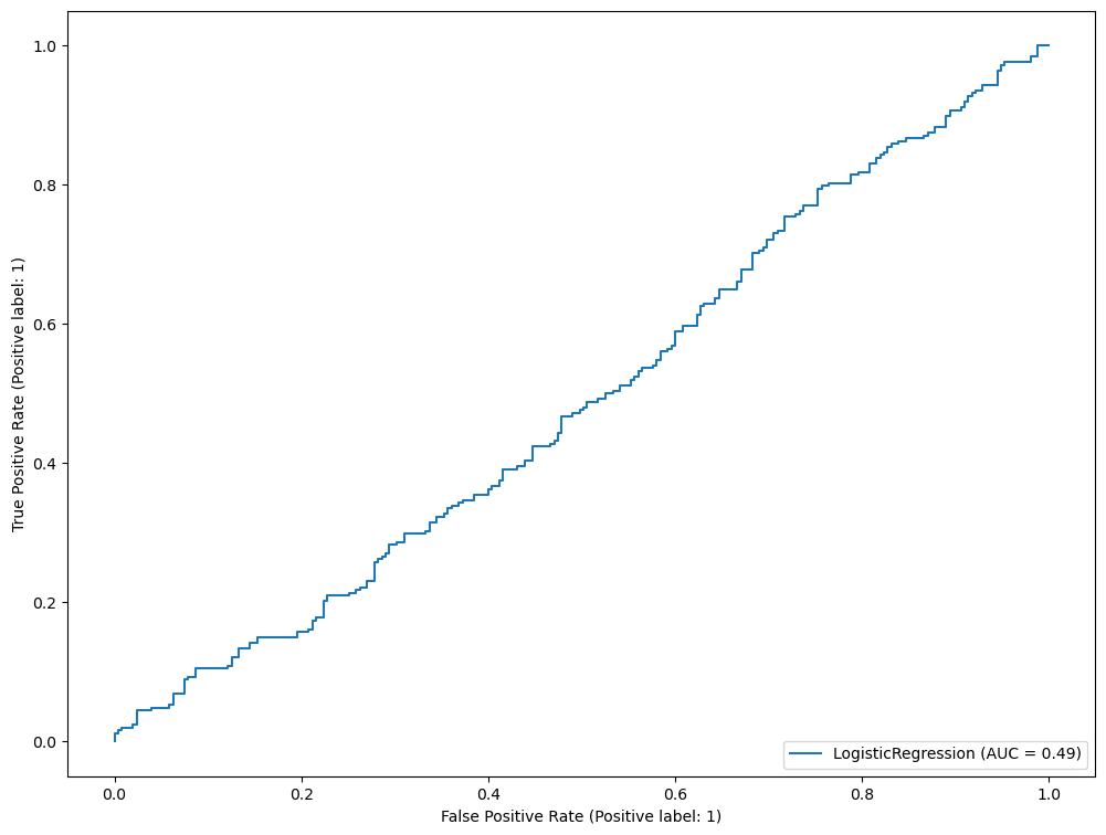

Decision Tree Classifier

Code

from sklearn.tree import DecisionTreeClassifier

# remember to use the random seed to be able to reproduce the same results
dt = DecisionTreeClassifier(random_state=RANDOM_SEED)
dt.fit(X_train, y_train)

RocCurveDisplay.from_estimator(dt, X_val, y_val)
#RocCurveDisplay.from_estimator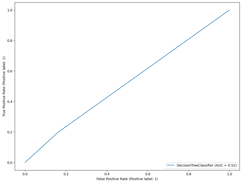

Random Forest

Code

from sklearn.ensemble import RandomForestClassifier

rf = RandomForestClassifier(random_state=RANDOM_SEED)
rf.fit(X_train, y_train)
RocCurveDisplay.from_estimator(rf, X_val, y_val)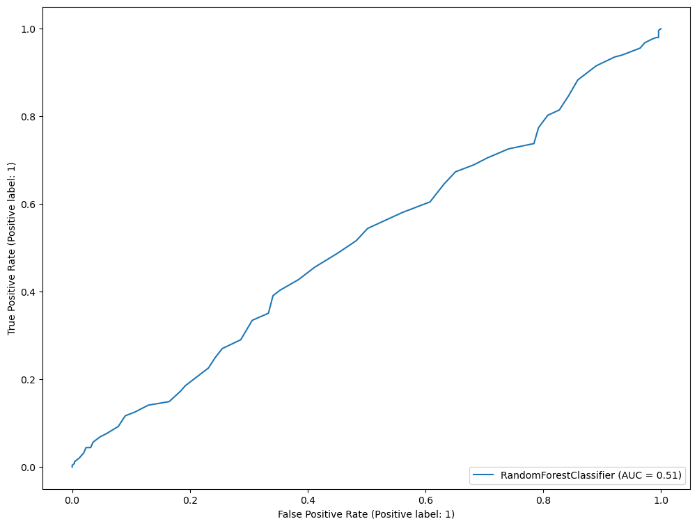

Gradient Boosting Ensemble

Code

from sklearn.ensemble import GradientBoostingClassifier

gb = GradientBoostingClassifier(random_state=RANDOM_SEED)
gb.fit(X_train, y_train)

RocCurveDisplay.from_estimator(gb, X_val, y_val)

Deep Learning Algorithm

Code

import tensorflow as tf

# set seed for reproducibility of results
tf.random.set_seed(RANDOM_SEED)

print("Tensorflow version", tf.__version__)

Tensorflow version 2.11.0

Code

model = tf.keras.models.Sequential([
    tf.keras.layers.Normalization(axis=-1),
    tf.keras.layers.Dense(10, input_shape=[X_train.shape[1],], activation="relu", kernel_initializer='random_normal', bias_initializer='zeros'),
    tf.keras.layers.Dropout(0.2, seed=RANDOM_SEED),
    tf.keras.layers.Dense(5, activation="relu", kernel_initializer='random_normal', bias_initializer='zeros'),
    tf.keras.layers.Dense(1, activation="sigmoid", kernel_initializer='random_normal', bias_initializer='zeros')
])

Code

# this configures the model's loss function, weight optimizer, and metrics to keep track of
model.compile(
    loss="binary_crossentropy", 
    optimizer=tf.keras.optimizers.Adam(), 
    metrics=['AUC']
)

Code

def learning_rate_scheduler(epoch, learning_rate):
    """Learning rate decay callback."""
    if epoch < 5:
        return learning_rate
    else:
        return learning_rate * tf.math.exp(-0.01)

early_stopping_callback = tf.keras.callbacks.EarlyStopping(patience=10, verbose=1, restore_best_weights=True)
learning_rate_callback = tf.keras.callbacks.LearningRateScheduler(learning_rate_scheduler)

Code

# the model.fit(...) method returns a 'history' object with stats about the training
history = model.fit(
    x=X_train,
    y=y_train,
    validation_data=(X_val, y_val),
    epochs=50,
    verbose=1,
    callbacks=[early_stopping_callback, learning_rate_callback])

Epoch 1/50
150/150 [==============================] - 1s 1ms/step - loss: 54.1560 - auc: 0.4979 - val_loss: 0.7589 - val_auc: 0.4888 - lr: 0.0010
Epoch 2/50
150/150 [==============================] - 0s 603us/step - loss: 1.9100 - auc: 0.5104 - val_loss: 0.6956 - val_auc: 0.4786 - lr: 0.0010
Epoch 3/50
150/150 [==============================] - 0s 589us/step - loss: 0.9015 - auc: 0.4972 - val_loss: 0.7808 - val_auc: 0.5095 - lr: 0.0010
Epoch 4/50
150/150 [==============================] - 0s 585us/step - loss: 0.7510 - auc: 0.5277 - val_loss: 0.6962 - val_auc: 0.4864 - lr: 0.0010
Epoch 5/50
150/150 [==============================] - 0s 592us/step - loss: 0.7006 - auc: 0.5049 - val_loss: 0.6948 - val_auc: 0.4911 - lr: 0.0010
Epoch 6/50
150/150 [==============================] - 0s 584us/step - loss: 0.7013 - auc: 0.5044 - val_loss: 0.6931 - val_auc: 0.5058 - lr: 9.9005e-04
Epoch 7/50
150/150 [==============================] - 0s 571us/step - loss: 0.6936 - auc: 0.5015 - val_loss: 0.6931 - val_auc: 0.5022 - lr: 9.8020e-04
Epoch 8/50
150/150 [==============================] - 0s 572us/step - loss: 0.6936 - auc: 0.4869 - val_loss: 0.6932 - val_auc: 0.4944 - lr: 9.7045e-04
Epoch 9/50
150/150 [==============================] - 0s 562us/step - loss: 0.6934 - auc: 0.4909 - val_loss: 0.6931 - val_auc: 0.5000 - lr: 9.6079e-04
Epoch 10/50
150/150 [==============================] - 0s 553us/step - loss: 0.6932 - auc: 0.4993 - val_loss: 0.6931 - val_auc: 0.5000 - lr: 9.5123e-04
Epoch 11/50
150/150 [==============================] - 0s 556us/step - loss: 0.6932 - auc: 0.4916 - val_loss: 0.6931 - val_auc: 0.5000 - lr: 9.4176e-04
Epoch 12/50
150/150 [==============================] - 0s 552us/step - loss: 0.6932 - auc: 0.5020 - val_loss: 0.6931 - val_auc: 0.5000 - lr: 9.3239e-04
Epoch 13/50
150/150 [==============================] - 0s 558us/step - loss: 0.6932 - auc: 0.4954 - val_loss: 0.6931 - val_auc: 0.5000 - lr: 9.2312e-04
Epoch 14/50
150/150 [==============================] - 0s 539us/step - loss: 0.6932 - auc: 0.5000 - val_loss: 0.6931 - val_auc: 0.5000 - lr: 9.1393e-04
Epoch 15/50
150/150 [==============================] - 0s 547us/step - loss: 0.6932 - auc: 0.5000 - val_loss: 0.6932 - val_auc: 0.5000 - lr: 9.0484e-04
Epoch 16/50
118/150 [======================>.......] - ETA: 0s - loss: 0.6932 - auc: 0.5000Restoring model weights from the end of the best epoch: 6.
150/150 [==============================] - 0s 575us/step - loss: 0.6932 - auc: 0.5000 - val_loss: 0.6932 - val_auc: 0.5000 - lr: 8.9583e-04
Epoch 16: early stopping

Code

model.summary()

Model: "sequential"
_________________________________________________________________
 Layer (type)                Output Shape              Param #   
=================================================================
 normalization (Normalizatio  (None, 10)               21        
 n)                                                              
                                                                 
 dense (Dense)               (None, 10)                110       
                                                                 
 dropout (Dropout)           (None, 10)                0         
                                                                 
 dense_1 (Dense)             (None, 5)                 55        
                                                                 
 dense_2 (Dense)             (None, 1)                 6         
                                                                 
=================================================================
Total params: 192
Trainable params: 171
Non-trainable params: 21
_________________________________________________________________

Code

from matplotlib import pyplot as plt

plt.plot(history.history['loss'], label='loss')
plt.plot(history.history['val_loss'], label='val_loss')
plt.xlabel('Epoch')
plt.ylabel('Error [Price]')
plt.legend()
plt.grid(True)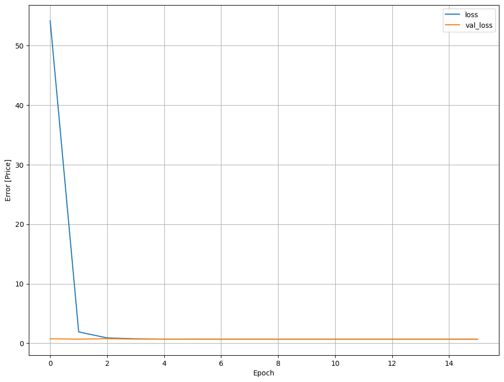

Code

plt.plot(history.history['auc'], label='auc')
plt.plot(history.history['val_auc'], label='val_auc')
plt.xlabel('Epoch')
plt.ylabel('Error [Price]')
plt.legend()
plt.grid(True)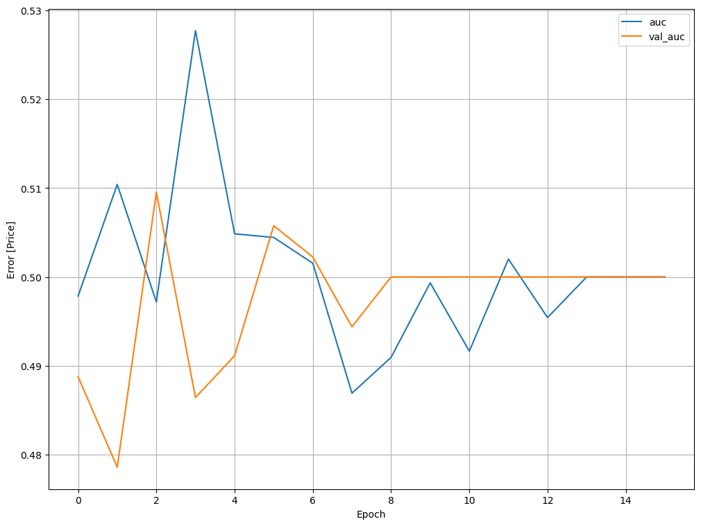

Conclusion

The gradient boosting classifier provided the best AUC score on the validation set. It is a common machine learning practice to train multiple models on the same train/validation data set and provide a model that works best. To simulate a production environment, we have held the test set aside until now.

Code

RocCurveDisplay.from_estimator(gb, X_test, y_test)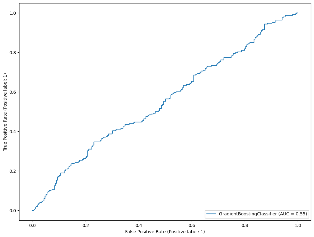

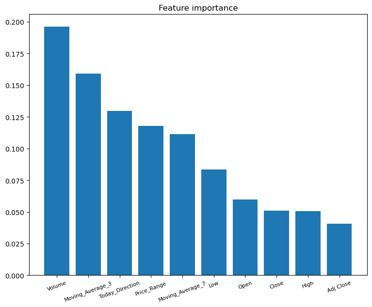
Code

import numpy as np
# Calculate feature importances
importances = gb.feature_importances_
# Sort feature importances in descending order
indices = np.argsort(importances)[::-1]

# Rearrange feature names so they match the sorted feature importances
names = [df_train[X_cols].columns[i] for i in indices]

_ = plt.figure(figsize=(9, 7))
plt.bar(names, importances[indices])
_ = plt.title("Feature importance")
_ = plt.xticks(rotation=20, fontsize = 8)