Finite-Difference Method - High-Order Taylor Operators

This exercise covers the following aspects

• Learn how to define high-order central finite-difference operators
• Investigate the behaviour of the operators with increasing length

Basic Equations

The Taylor expansion of \(f(x + dx)\) around \(x\) is defined as

\[ f(x+dx)=\sum_{n=0}^\infty \frac{f^{(n)}(x)}{n!}dx^{n} \]

Finite-difference operators can be calculated by seeking weights (here: \(a\), \(b\), \(c\)) with which function values have to be multiplied to obtain an interpolation or a derivative. Example:

\[ \begin{align} a ~ f(x + dx) & \ = \ a ~ \left[ ~ f(x) + f^{'} (x) dx + \frac{1}{2!} f^{''} (x) dx^2 + \dotsc ~ \right] \\ b ~ f(x) & \ = \ b ~ \left[ ~ f(x) ~ \right] \\ c ~ f(x - dx) & \ = \ c ~ \left[ ~ f(x) - f^{'} (x) dx + \frac{1}{2!} f^{''} (x) dx^2 - \dotsc ~ \right] \end{align} \]

This can be expressed in matrix form by comparing coefficients, here seeking a 2nd derivative

\[ \begin{align} &a ~~+~~ ~~~~b &+~~ c & = & 0 \\ &a ~~\phantom{+}~~ \phantom{b} &-~~ c & = & 0 \\ &a ~~\phantom{+}~~ \phantom{b} &+~~ c & = & \frac{2!}{\mathrm{d}x^2} \end{align} \]

which leads to

\[ \begin{pmatrix} 1 & 1 & 1 \\ 1 & 0 & -1 \\ 1 & 0 & 1 \end{pmatrix} \begin{pmatrix} a\\ b \\ c \end{pmatrix} = \begin{pmatrix} 0\\ 0 \\ \frac{2!}{dx^2} \end{pmatrix} \]

and using matrix inversion we obtain

\[ \begin{pmatrix} a \\ b\\ c \end{pmatrix} = \begin{pmatrix} \frac{1}{2 \mathrm{d}x^2} \\ - \frac{2}{2 \mathrm{d}x^2} \\ \frac{1}{2 \mathrm{d}x^2} \end{pmatrix} \]

This is the the well known 3-point operator for the 2nd derivative. This can easily be generalized to higher point operators and higher order derivatives. Below you will find a routine that initializes the system matrix and solves for the Taylor operator.

Calculating the Taylor operator

The subroutine central_difference_coefficients() initializes the system matrix and solves for the difference weights assuming \(dx=1\). It calculates the centered differences using an arbitrary number of coefficients, also for higher derivatives. The weights are defined at \(x\pm i dx\) and \(i=0,..,(nop-1)/2\), where \(nop\) is the length of the operator. Careful! Because it is centered \(nop\) has to be an odd number (3,5,…)!

It returns a central finite difference stencil (a vector of length \(nop\)) for the nth derivative.

# Import libaries
import math
import numpy as np
import matplotlib.pyplot as plt

# Define function to calculate Taylor operators
def central_difference_coefficients(nop, n):
    """
    Calculate the central finite difference stencil for an arbitrary number
    of points and an arbitrary order derivative.
    
    :param nop: The number of points for the stencil. Must be
        an odd number.
    :param n: The derivative order. Must be a positive number.
    """
    m = np.zeros((nop, nop))
    for i in range(nop):
        for j in range(nop):
            dx = j - nop // 2
            m[i, j] = dx ** i
    
    s = np.zeros(nop)
    s[n] = math.factorial(n)
    
    # The following statement return oper = inv(m) s
    oper = np.linalg.solve(m, s)
    # Calculate operator
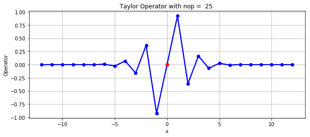
    return oper

Plot Taylor operators

Investigate graphically the Taylor operators. Increase \(nop\) for the first \(n=1\) or higher order derivatives. Discuss the results and try to understand the interpolation operator (derivative order \(n=0\)).

# Calculate and plot Taylor operator

# Give length of operator (odd)
nop = 25
# Give order of derivative (0 - interpolation, 1 - first derivative, 2 - second derivative)
n = 1

# Get operator from routine 'central_difference_coefficients'
oper = central_difference_coefficients(nop, n)

# Plot operator
x = np.linspace(-(nop - 1) / 2, (nop - 1) / 2, nop)

# Simple plot with operator
plt.figure(figsize=(10, 4))
plt.plot(x, oper,lw=2,color='blue')
plt.plot(x, oper,lw=2,marker='o',color='blue')
plt.plot(0, 0,lw=2,marker='o',color='red')
#plt.plot (x, nder5-ader, label="Difference", lw=2, ls=":")
plt.title("Taylor Operator with nop =  %i " % nop )
plt.xlabel('x')
plt.ylabel('Operator')
plt.grid()
plt.show()

Conclusions

• The Taylor operator weights decrease rapidly with distance from the central point
• In practice often 4th order operators are used to calculate space derivatives