Numerical derivative and comparison with analytical solution

This exercise covers the following aspects:

• Calculation of numerical first derivative
• Comparison with analytical solution
• Dependence of error on space increment

Note: Alternative solution added that looks at the convergence by decreasing the spatial increment dx (May 12, 2020)

# Import Libraries
import numpy as np
from math import *
import matplotlib.pyplot as plt

We initialize a space-dependent sin function

\[\begin{equation} f(x)= \sin (k x) \end{equation}\]

where the wavenumber k is

\[\begin{equation} k = \dfrac{2 \pi}{\lambda} \end{equation}\]

and \(\lambda\) is wavelength.

# Initial parameters
xmax = 10.0                     # physical domain (m)
nx = 200                        # number of samples    
dx = xmax/(nx-1)                # grid increment dx (m)
x  = np.linspace(0,xmax,nx)     # space coordinates

# Initialization of sin function
l = 40*dx     # wavelength
k = 2*pi/l    # wavenumber
f = np.sin(k*x)
l,k

(2.0100502512562817, 3.125884690321844)

# Plot sin function
plt.figure(figsize=(10,6))
plt.plot(x, f)
plt.title('Sin function')
plt.xlabel('x, m')
plt.ylabel('Amplitude')
plt.xlim((0, xmax))
plt.grid()
plt.show()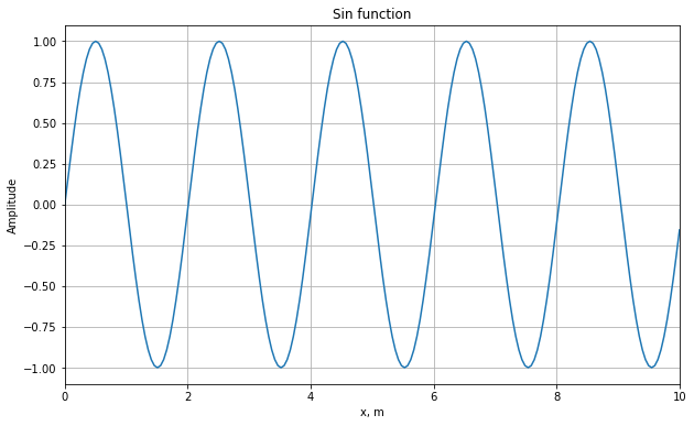

In the cell below we calculate the central finite-difference derivative of f(x) using two points

\[\begin{equation} f^{\prime}(x)=\dfrac{f(x+dx)-f(x-dx)}{2dx} \end{equation}\]

and compare with the analytical derivative

\[\begin{equation} f^{\prime}(x) = k \cos(k x) \end{equation}\]

# First derivative with two points

# Initiation of numerical and analytical derivatives 
nder=np.zeros(nx)          # numerical derivative
ader=np.zeros(nx)          # analytical derivative

# Numerical derivative of the given function
for i in range (1, nx-1):
    nder[i]=(f[i+1]-f[i-1])/(2*dx)

# Analytical derivative of the given function
ader= k * np.cos(k*x)   
# Exclude boundaries
ader[0]=0.
ader[nx-1]=0.

# Error (rms) 
rms = np.sqrt(np.mean((nder-ader)**2))

# Plotting 
# ----------------------------------------------------------------
plt.figure(figsize=(10,6))
plt.plot (x, nder,label="Numerical Derivative, 2 points", marker='+', color="blue")
plt.plot (x, ader, label="Analytical Derivative", lw=2, ls="-",color="black")
plt.plot (x, nder-ader, label="Difference", lw=2, ls=":")
plt.title("First derivative, Err (rms) = %.6f " % (rms) )
plt.xlabel('x, m')
plt.ylabel('Amplitude')
plt.legend(loc='lower left')
plt.grid()
plt.show()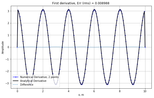

The concept of number of points per wavelength

\[\begin{equation} n_\lambda = \dfrac{\lambda}{dx} \end{equation}\]

How does the error of the numerical derivative change with the number of points per wavelength?

# Plotting number of points per wavelength
plt.figure(figsize=(10,6))
plt.plot (x, nder,label="Numerical Derivative, 2 points", marker='+', color="blue")
plt.title("First derivative, Error = %.6f, $n_\lambda$ = %.2f " % ( rms, l/dx) )
plt.xlabel('x, m')
plt.ylabel('Amplitude')
plt.legend(loc='lower left')
plt.xlim((xmax/2-l,xmax/2+l))
plt.grid()
plt.show()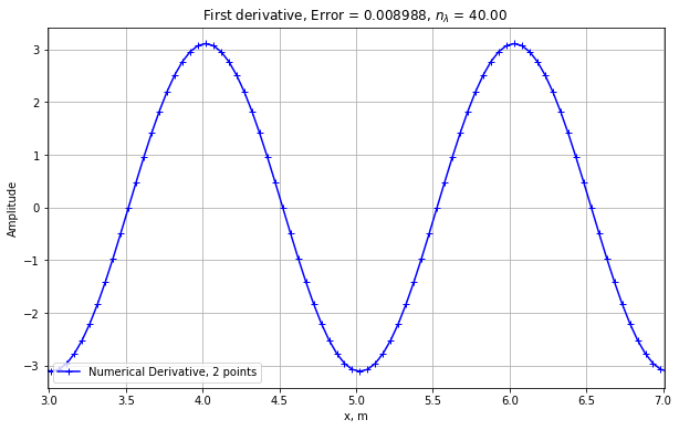

Investigate the error as a function of grid points per wavelength

# Define a range of number of points per wavelength: [nmin=4,5,6 ... ,nmax=40]
# Loop over points, calculate corresponding wavelength and calculate error

# Initialize vectors
nmin=3
nmax=40
na =  np.zeros(nmax-nmin+1)    # Vector with number of points per wavelength
err = np.zeros(nmax-nmin+1)    # Vector with error

j = -1  # array index


# Loop through finite-difference derivative calculation
for n in range (nmin,nmax+1):
    
    j = j+1   # array index
    na[j] = n

    
    # Initialize sin function
    l = na[j]*dx  # wavelength
    k = 2*pi/l    # wavenumber
    f = np.sin(k*x)

    # Numerical derivative of the sin function
    for i in range (1, nx-1):
        nder[i]=(f[i+1]-f[i-1])/(2*dx)

    # Analytical derivative of the sin function
    ader= k * np.cos(k*x)   
    # Exclude boundaries
    ader[0]=0.
    ader[nx-1]=0.

    # Error (rms) 
    err[j] = np.sum((nder-ader)**2)/np.sum((ader**2)) * 100

# ----------------------------------------------------------------
# Plotting error as function of number of points per wavelength
plt.figure(figsize=(10,6))
plt.plot(na,err, ls='-', color="blue")
plt.title('Error as a function of $n_\lambda$ ')
plt.xlabel('n$_\lambda$')
plt.ylabel('rms ')
plt.grid()
plt.show()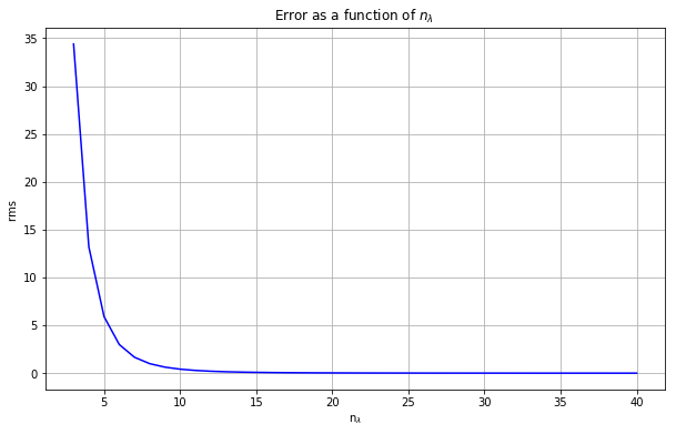

Alternative Solution (as requested by several comments):

Let us fix the wavelength lambda and decrease the spatial increment \(dx\) and by that increasing the number of points per wavelength. To make it compatible with the Nyquist theorem we start the discretization close to the Nyquist wavelength \(\lambda_{Ny} = 2 dx\).

# Let us loop over number of points in the interval [5,100], 3 points corresponds to Nyquist wavelength

n1 =5
n2 =100
err = np.zeros(n2-n1-1)   # vector for error
dxa = np.zeros(n2-n1-1)   # vector for dx
npl = np.zeros(n2-n1-1)   # vector for number of points per lambda


ii = -1 

for n in range (n1,n2-1):
    ii   = ii + 1
    x    = np.linspace(0,2*np.pi,n)
    dx   = x[1]-x[0]
    f    = np.sin(x)
    df   = np.cos(x)     # Analytical derivative
    
    dfn = np.zeros(n)
    # Numerical derivative of the sin function
    for i in range (1, n-1):
        dfn[i]=(f[i+1]-f[i-1])/(2*dx)
    
    # Calculate error in the interval in which numerical derivative was calculated
    err[ii] = np.sum((df[1:n-1]-dfn[1:n-1])**2)/np.sum((df[1:n-1]**2)) * 100 
    
    dxa[ii] = dx         # dx
    npl[ii] = 2*np.pi/dx # number of points per wavelength
    

# ----------------------------------------------------------------
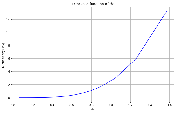
# Plotting error as function of dx
plt.figure(figsize=(10,6))
plt.plot(dxa,err, ls='-', color="blue")
plt.title('Error as a function of $dx$ ')
plt.xlabel('dx')
plt.ylabel('Misfit energy (%) ')
plt.grid()
plt.show()

# ----------------------------------------------------------------
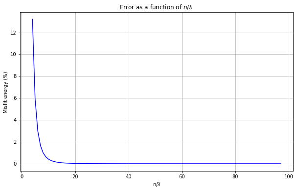
# Plotting error as function of points per wavelength
plt.figure(figsize=(10,6))
plt.plot(npl,err, ls='-', color="blue")
plt.title('Error as a function of $n/\lambda$ ')
plt.xlabel('n/$\lambda$')
plt.ylabel('Misfit energy (%) ')
plt.grid()
plt.show()
    

Conclusions

• 2-point finite-difference approximations can provide estimates of the 1st derivative of a function
• The accuracy depends on the “number of points per wavelength”, i.e., how well we sample the original function
• The more points per wavelength we use the more accurate is the derivative approximation