Weakly-Supervised Deep Learning for Cancer Diagnosis in Computational Pathology

Background: Tissue phenotyping is a fundamental problem in computational pathology (CPATH) to characterize histopathologic features within gigapixel whole-slide images (WSIs) for cancer diagnosis, prognosis, and prediction of treatment response. Unlike natural images, whole-slide imaging is a challenging computer vision domain in which image resolutions can be as large as \(150{,}000 \times 150{,}000\) pixels, with many methods using the following three-stage, weakly-supervised framework based on multiple instance learning (MIL): 1) tissue patching at a single magnification objective (“zoom”), 2) patch-level feature extraction to construct a sequence of embedding instances, and 3) global pooling of instances to construct a slide-level representation for weak-supervision using slide-level labels (e.g., subtype, grade, stage, survival, origin).

Notebook Objective: The following exercise is based on the Lung Adenocarcinoma (LUAD) vs. Lung Squamous Cell Carcinoma (LUSC) subtyping task used in experimental setup in Lu et al., Data-efficient and weakly supervised computational pathology on whole-slide images Nature BME 2021 and it’s open-sourced codebase on GitHub, CLAM, in which we will: 1. Train and evaluate a “naive” MIL algorithm called AverageMIL, which takes the average of patch embeddings (as the global pooling operator). A minimalistic but fully-implemented training setup in PyTorch is provided. 2. Implement a more sophisticated algorithm called Attention-Based Multiple Instance Learning (ABMIL), which learns attention weights for computing a weighted average of patch embeddings. 3. Compare and contrast AverageMIL and ABMIL, discussing which algorithm performs better and potential limitations.

About this notebook: - Model implementation and training is directly adapted from CLAM, with many additional features (e.g. - letting users set up optimizers, model types, logging information, and other hyper-parameters) left out due to making this notebook as simple to run as possible for teaching purposes. To use all features, please see CLAM. - Though this notebook is based off of CLAM, the method-of-interest that you will be implementing is not CLAM, but a different method called ABMIL from Ilse et al. Attention-Based Multiple Instance Learning ICML 2018, which CLAM is derived from. The main reason why ABMIL is used over CLAM is due to code length (ABMIL can be written in less than 20 lines). - Though pre-extracted features were generated using the CLAM codebase, the encoder was not a truncated ResNet-50 pretrained on ImageNet (dimension 1024) at 20 \(\times\) resolution. Instead, we extracted features with a much smaller CNN encoder (dimension 320) at 10 \(\times\) resolution, which shrinks the size of the dataset from ~11 GB to ~3.96 GB of storage (download link for pre-extracted features in the cell below) and thus allows you to easily train this model using your CPU (no GPU required!). In addition, a torch.seed is set for reproducibility (all outputs should be deterministic).

Colab Installation, Data Download, & Dependencies

Code
# gets clinical metadata csv for tcga-luad and tcga-lusc with predefined train/val/test splits
# gets pre-extracted features for tcga-luad and tcga-lusc diagnostic WSIs (1043 WSIs total, ~3.96 GB in size, ~67 seconds to download)
# alternatively, you can download the data directly from Dropbox to your local computer, and run this Colab Notebook locally
!wget https://www.dropbox.com/s/5wuvu791vwntg9o/tcga_lung_splits.csv
!wget https://www.dropbox.com/s/euepd2owxvuwr7v/feats_pt.zip
!unzip -q feats_pt.zip
--2024-04-24 18:44:17--  https://www.dropbox.com/s/5wuvu791vwntg9o/tcga_lung_splits.csv
Resolving www.dropbox.com (www.dropbox.com)... 162.125.6.18, 2620:100:6019:18::a27d:412
Connecting to www.dropbox.com (www.dropbox.com)|162.125.6.18|:443... connected.
HTTP request sent, awaiting response... 302 Found
Location: /s/raw/5wuvu791vwntg9o/tcga_lung_splits.csv [following]
--2024-04-24 18:44:18--  https://www.dropbox.com/s/raw/5wuvu791vwntg9o/tcga_lung_splits.csv
Reusing existing connection to www.dropbox.com:443.
HTTP request sent, awaiting response... 302 Found
Location: https://uc00b78a030854673fbbe33a21fa.dl.dropboxusercontent.com/cd/0/inline/CRosyqWmLZhYHRD7UhsN1FO8xLIoX_Ws9Vr81jPF23t7CediZcwYRmfziuAnNPP4GqsEw4RVIV_8FjtiFHHMd5N0JXmo2nWoL-ObiXARX0Eo9thV8w-peRUOjIDmu7n5QDS3hx5f4CDU7mHt3R3a0QQK/file# [following]
--2024-04-24 18:44:18--  https://uc00b78a030854673fbbe33a21fa.dl.dropboxusercontent.com/cd/0/inline/CRosyqWmLZhYHRD7UhsN1FO8xLIoX_Ws9Vr81jPF23t7CediZcwYRmfziuAnNPP4GqsEw4RVIV_8FjtiFHHMd5N0JXmo2nWoL-ObiXARX0Eo9thV8w-peRUOjIDmu7n5QDS3hx5f4CDU7mHt3R3a0QQK/file
Resolving uc00b78a030854673fbbe33a21fa.dl.dropboxusercontent.com (uc00b78a030854673fbbe33a21fa.dl.dropboxusercontent.com)... 162.125.6.15, 2620:100:601c:15::a27d:60f
Connecting to uc00b78a030854673fbbe33a21fa.dl.dropboxusercontent.com (uc00b78a030854673fbbe33a21fa.dl.dropboxusercontent.com)|162.125.6.15|:443... connected.
HTTP request sent, awaiting response... 200 OK
Length: 170283 (166K) [text/plain]
Saving to: ‘tcga_lung_splits.csv’

tcga_lung_splits.cs 100%[===================>] 166.29K  --.-KB/s    in 0.005s  

2024-04-24 18:44:18 (31.2 MB/s) - ‘tcga_lung_splits.csv’ saved [170283/170283]

--2024-04-24 18:44:19--  https://www.dropbox.com/s/euepd2owxvuwr7v/feats_pt.zip
Resolving www.dropbox.com (www.dropbox.com)... 162.125.6.18, 2620:100:6019:18::a27d:412
Connecting to www.dropbox.com (www.dropbox.com)|162.125.6.18|:443... connected.
HTTP request sent, awaiting response... 302 Found
Location: /s/raw/euepd2owxvuwr7v/feats_pt.zip [following]
--2024-04-24 18:44:19--  https://www.dropbox.com/s/raw/euepd2owxvuwr7v/feats_pt.zip
Reusing existing connection to www.dropbox.com:443.
HTTP request sent, awaiting response... 302 Found
Location: https://ucf014afc0b6c260bbb67dbd7452.dl.dropboxusercontent.com/cd/0/inline/CRrKpEw8EBgkTnISQM7LLM3urYUBFzI76SZUKCdT7P8ZYt1c8gH9w-HCjFBTc5JQah06yFZIdJv-bPdLbGySHBH2C8PH-o-45yftS03TNmPgpfoopk4C3mRsUa3j6OdY5YmIiyw5dlk-qUePY3q9vVPF/file# [following]
--2024-04-24 18:44:20--  https://ucf014afc0b6c260bbb67dbd7452.dl.dropboxusercontent.com/cd/0/inline/CRrKpEw8EBgkTnISQM7LLM3urYUBFzI76SZUKCdT7P8ZYt1c8gH9w-HCjFBTc5JQah06yFZIdJv-bPdLbGySHBH2C8PH-o-45yftS03TNmPgpfoopk4C3mRsUa3j6OdY5YmIiyw5dlk-qUePY3q9vVPF/file
Resolving ucf014afc0b6c260bbb67dbd7452.dl.dropboxusercontent.com (ucf014afc0b6c260bbb67dbd7452.dl.dropboxusercontent.com)... 162.125.6.15, 2620:100:6019:15::a27d:40f
Connecting to ucf014afc0b6c260bbb67dbd7452.dl.dropboxusercontent.com (ucf014afc0b6c260bbb67dbd7452.dl.dropboxusercontent.com)|162.125.6.15|:443... connected.
HTTP request sent, awaiting response... 302 Found
Location: /cd/0/inline2/CRrFzRNAP_XORwY2Kgzmc_DiBxpq4PsX2TbQ6M-YqHRS8scIE3nuQEQkenws5Qols-IsveCYeRvWYFrTSvLNi2apchZrl7zoDPCnnJPM2HEPnYz8NrohrEZ9ivYkbBJ5Wf-0_zzj2pwPJjp5p_Uw0FQFUnNdMOY7TsHfT-Tl1zRJPEnIt914OIZPorornUQNyRM82h80E311CuaYHoF-u0Nms70UAIirzLjB8YmjOKBAyIAqJWVwB4L-YSYvCD1d-mraSusuYdJd5F_LqtsjJ-mfOnRIfGdLYfvDx0bQ3uTyg8N9v7DNpFBTsxwOhtQPq-9j8JeDJDyKDzOeRZcUn20zhASusSkrpod3oZgOH4oSvPO2AC0gINHPqYA0MPjH7ig/file [following]
--2024-04-24 18:44:20--  https://ucf014afc0b6c260bbb67dbd7452.dl.dropboxusercontent.com/cd/0/inline2/CRrFzRNAP_XORwY2Kgzmc_DiBxpq4PsX2TbQ6M-YqHRS8scIE3nuQEQkenws5Qols-IsveCYeRvWYFrTSvLNi2apchZrl7zoDPCnnJPM2HEPnYz8NrohrEZ9ivYkbBJ5Wf-0_zzj2pwPJjp5p_Uw0FQFUnNdMOY7TsHfT-Tl1zRJPEnIt914OIZPorornUQNyRM82h80E311CuaYHoF-u0Nms70UAIirzLjB8YmjOKBAyIAqJWVwB4L-YSYvCD1d-mraSusuYdJd5F_LqtsjJ-mfOnRIfGdLYfvDx0bQ3uTyg8N9v7DNpFBTsxwOhtQPq-9j8JeDJDyKDzOeRZcUn20zhASusSkrpod3oZgOH4oSvPO2AC0gINHPqYA0MPjH7ig/file
Reusing existing connection to ucf014afc0b6c260bbb67dbd7452.dl.dropboxusercontent.com:443.
HTTP request sent, awaiting response... 200 OK
Length: 3961539230 (3.7G) [application/zip]
Saving to: ‘feats_pt.zip’

feats_pt.zip        100%[===================>]   3.69G  96.5MB/s    in 52s     

2024-04-24 18:45:13 (72.3 MB/s) - ‘feats_pt.zip’ saved [3961539230/3961539230]
Code
import os
import copy
import matplotlib.pyplot as plt
import seaborn
import numpy as np
import pandas as pd
import sklearn.metrics
import torch
import torch.nn as nn
import torch.nn.functional as F
import torchvision
print(torch.__version__)
2.2.1+cu121

(Primer) WSI Data Preprocessing for Histology Slides in the TCGA-Lung Cohort

To process WSIs, tools such as CLAM are typically used for tissue patching and non-overlapping patch feature extraction. Though easy-to-use, using CLAM for feature processing would require downloading gigapixel WSIs (> 1000 WSIS in TCGA-LUAD and TCGA-LUSC), which exceeds over >100GB of storage space. To alleviate this issue, this problem set provides pre-extracted features (processed via CLAM, but using a much smaller vision encoder with \(D = 320\)). However, to still illustrate how CLAM preprocessing works, the cell below describes a high-level overview on how WSIs are formulated as [M x D]-dim bag of patch embeddings, where M is the number of tissue patches and D is the hidden dimension size of your encoder. Again, please use CLAM if you are interested in re-generating these features.

Code
# Let's say we have a "bag" of M [256 x 256 x 3] image patches (M = 512), which are taken from non-overlapping patches in the WSI.
M = 512
X = torch.randn(M, 3, 256, 256) # Arranged in (Batch, Channel, Width, Height) format or (B, C, W, H) for short
print("WSI Shape:", X.shape)

# We would typically use a CNN model (pretrained on ImageNet) as our vision encoder for pre-extracting "dense, intermediate" features from each patch
cnn = torchvision.models.mobilenet_v3_small()
cnn.eval()

# Since this model was taken from torchvision and trained on ImageNet, the output of the model are the probability scores of the ImageNet classes (1000 classes total).
# To extract useful features from each patch, we have to use the penultimate layer(s) of the CNN, before feeding it into a linear layer.
print("Probability Scores for ImageNet:", cnn.forward(X[:1]).shape)

# To extract the penultimate features, we can define a new function that returns the features
# before giving it to internal classifier layer within the model.
# Again, we want to use the pretrained features on ImageNet, but don't want the classification scores for "ImageNet" classes!
# # See the below documentation for how the forward pass in MobileNetV3 works.
# https://pytorch.org/vision/main/_modules/torchvision/models/mobilenetv3.html#mobilenet_v3_small
encoder = lambda x: torch.flatten(cnn.avgpool(cnn.features(x)), 1)
print("Feature Embedding Shape:", encoder(X[:1]).shape)

# We can now use our encoder to extract features for each patch.
# Typically, the # of non-overlapping patches in a WSI is ~15,000. Thus, we often have to extract patch features in mini-batches.
batch_size = 32
H = []
for bag_idx in range(0, M, batch_size):
    H.append(encoder(X[bag_idx:(bag_idx+batch_size)]).cpu().detach().numpy())
print("Bag Shape", np.vstack(H).shape)
WSI Shape: torch.Size([512, 3, 256, 256])
Probability Scores for ImageNet: torch.Size([1, 1000])
Feature Embedding Shape: torch.Size([1, 576])
Bag Shape (512, 576)

(Primer) Data Exploration

Code
# where we downloaded the features and label csv to
feats_dirpath, csv_fpath = './feats_pt/', './tcga_lung_splits.csv'

# label csv matches case_id (patient), slide_id (WSI image filename), and diagnosis (LUAD vs LUSC)
# as well as pre-defined splits (train / val / test)
df = pd.read_csv(csv_fpath)
display(df)
display(df[['split', 'OncoTreeCode']].value_counts())

# extracted feature filenames + slide_id column match
feats_pt_fnames = pd.Series(os.listdir(feats_dirpath))
print("Example filenames for extracted features:", list(feats_pt_fnames[:5]))
print("Overlap of extracted feature filenames + slide_id column:",
      len(set(df['slide_id']).intersection(set(feats_pt_fnames.str[:-3]))))

# statistics about the size of each bag
bag_sizes = []
for e in os.scandir(feats_dirpath):
    feats_pt = torch.load(e.path)    # [M x d]-dim tensor
    bag_sizes.append(feats_pt.shape[0])
print('Mean Bag Size:', np.mean(bag_sizes))
print('Std Bag Size:', np.std(bag_sizes))
case_id slide_id tumor_type OncoTreeSiteCode main_cancer_type sex project_id Diagnosis OncoTreeCode OncoTreeCode_Binarized split
0 TCGA-73-4676 TCGA-73-4676-01Z-00-DX1.4d781bbc-a45e-4f9d-b6b... Primary LUNG Non-Small Cell Lung Cancer M TCGA-LUAD Lung Adenocarcinoma LUAD 0 train
1 TCGA-MP-A4T6 TCGA-MP-A4T6-01Z-00-DX1.085C4F5A-DB1B-434A-9D6... Primary LUNG Non-Small Cell Lung Cancer F TCGA-LUAD Lung Adenocarcinoma LUAD 0 train
2 TCGA-78-7167 TCGA-78-7167-01Z-00-DX1.f79e1a9b-a3eb-4c91-a1f... Primary LUNG Non-Small Cell Lung Cancer M TCGA-LUAD Lung Adenocarcinoma LUAD 0 train
3 TCGA-L9-A444 TCGA-L9-A444-01Z-00-DX1.88CF6F01-0C1F-4572-81E... Primary LUNG Non-Small Cell Lung Cancer F TCGA-LUAD Lung Adenocarcinoma LUAD 0 train
4 TCGA-55-8097 TCGA-55-8097-01Z-00-DX1.2f847b65-a5dc-41be-9dd... Primary LUNG Non-Small Cell Lung Cancer F TCGA-LUAD Lung Adenocarcinoma LUAD 0 train
... ... ... ... ... ... ... ... ... ... ... ...
1038 TCGA-21-A5DI TCGA-21-A5DI-01Z-00-DX1.E9123261-ADE7-468C-9E9... Primary LUNG Non-Small Cell Lung Cancer M TCGA-LUSC Lung Squamous Cell Carcinoma LUSC 1 test
1039 TCGA-77-7465 TCGA-77-7465-01Z-00-DX1.25e4b0b4-4948-432f-801... Primary LUNG Non-Small Cell Lung Cancer M TCGA-LUSC Lung Squamous Cell Carcinoma LUSC 1 test
1040 TCGA-34-8454 TCGA-34-8454-01Z-00-DX1.A2308ED3-E430-4448-853... Primary LUNG Non-Small Cell Lung Cancer F TCGA-LUSC Lung Squamous Cell Carcinoma LUSC 1 test
1041 TCGA-77-7138 TCGA-77-7138-01Z-00-DX1.8c912762-0829-4692-92a... Primary LUNG Non-Small Cell Lung Cancer M TCGA-LUSC Lung Squamous Cell Carcinoma LUSC 1 test
1042 TCGA-77-8131 TCGA-77-8131-01Z-00-DX1.dcb8e2c7-0d2f-4b38-9db... Primary LUNG Non-Small Cell Lung Cancer M TCGA-LUSC Lung Squamous Cell Carcinoma LUSC 1 test

1043 rows × 11 columns

split  OncoTreeCode
train  LUAD            433
       LUSC            415
test   LUAD             49
       LUSC             49
val    LUAD             49
       LUSC             48
Name: count, dtype: int64
Example filenames for extracted features: ['TCGA-33-A4WN-01Z-00-DX1.438D0EF6-C329-41E5-A7D5-7F037DE34106.pt', 'TCGA-77-7465-01Z-00-DX1.25e4b0b4-4948-432f-8010-a6c6e4652cab.pt', 'TCGA-98-A53H-01Z-00-DX1.B05E6339-440C-4F2E-95B5-F2C96413D488.pt', 'TCGA-55-8512-01Z-00-DX1.FD4B9CF5-1955-420E-A955-6D284772D2BE.pt', 'TCGA-86-6562-01Z-00-DX1.5dea3015-e606-4837-9f99-ac14f0aa091b.pt']
Overlap of extracted feature filenames + slide_id column: 1043
Mean Bag Size: 3259.9090038314175
Std Bag Size: 2133.97437395412

Question 1. Visualizing Performance Metrics for AverageMIL (15 points)

Implemented in the Google Colab notebook is a minimalistic training setup that performs weakly-supervised learning via AverageMIL on LUAD vs. LUSC subtyping using 1043 diagnostic H&E tissue slides from the The Cancer Genome Atlas (features already pre-extracted and downloaded from Colab installation, clinical metadata for all case and slide IDs also downloaded). You can run the cells in the Google Colab Notebook and see how well this algorithm performs in 20 epochs. Though fully implemented, some performance metrics are missing which would help you understand how well this model performs. 1. In the current implementation, only the epoch loss, balanced accuracy, and overall AUC is tracked. In addition to these metrics, calculate and log the per-class accuracy (per epoch) in the traineval_epoch function. 2. For the above metrics (loss, balanced ACC, per-class ACC, overall AUC), visualize the train and validation performance for 20 epochs (or until early stopping) using packages such as matplotlib, seaborn, and other appropriate plotting packages. Each metric should have its own separate plot (x-axis = epochs, y-axis = metric), and show curves for both train and validation.

Code
class AverageMIL(nn.Module):
    def __init__(self, input_dim=320, hidden_dim=64, dropout=0.25, n_classes=2):
        r"""
        AverageMIL, a naive MIL algorithm that average pools all patch features.

        Args:
            input_dim (int): input feature dimension.
            hidden_dim (int): hidden layer dimension.
            dropout (float): Dropout probability.
            n_classes (int): Number of classes.
        """
        super(AverageMIL, self).__init__()
        self.inst_level_fc = nn.Sequential(*[nn.Linear(input_dim, hidden_dim),
                                             nn.ReLU(),
                                             nn.Dropout(dropout)]) # Fully-Connected Layer, applied "instance-wise" to each embedding
        self.bag_level_classifier = nn.Linear(hidden_dim, n_classes)                                            # Bag-Level Classifier

    def forward(self, H: torch.randn(100, 320)):
        r"""
        Takes as input a [M x D]-dim bag of patch features (representing a WSI), and outputs: 1) logits for classification, 2) un-normalized attention scores.

        Args:
            H (torch.Tensor): [M x D]-dim bag of patch features (representing a WSI)

        Returns:
            logits (torch.Tensor): [1 x n_classes]-dim tensor of un-normalized logits for classification task.
            None (no attention scores to return)
        """
        H = self.inst_level_fc(H)                   # 1. Preprocesses each "instance-level" embedding to be "hidden-dim"-dim size
        z = H.mean(dim=0).unsqueeze(dim=0)          # 2. Average of Patch Embeddings
        logits = self.bag_level_classifier(z)       # 3. Bag-Level Classifier
        return logits, None


class MILDataset(torch.utils.data.dataset.Dataset):
    r"""
    torch.utils.data.dataset.Dataset object that loads pre-extracted features per WSI from a CSV.

    Args:
        feats_dirpath (str): Path to pre-extracted patch features (assumes that these features are saved as a *.pt object with it's corresponding slide_id as the filename)
        csv_fpath (str): Path to CSV file which contains: 1) Case ID, 2) Slide ID, 3) split information (train / val / test), and 4) label columns of interest for classification.
        which_split (str): Split that is used for subsetting the CSV (choices: ['train', 'val', 'test'])
        n_classes (int): Number of classes (default == 2 for LUAD vs LUSC subtyping)
    """
    def __init__(self, feats_dirpath='./', csv_fpath='./tcga_lung_splits.csv', which_split='train', which_labelcol='OncoTreeCode_Binarized'):
        self.feats_dirpath, self.csv, self.which_labelcol = feats_dirpath, pd.read_csv(csv_fpath), which_labelcol
        self.csv_split = self.csv[self.csv['split']==which_split]

    def __getitem__(self, index):
        features = torch.load(os.path.join(self.feats_dirpath, self.csv_split.iloc[index]['slide_id']+'.pt'))
        label = self.csv_split.iloc[index][self.which_labelcol]
        return features, label

    def __len__(self):
        return self.csv_split.shape[0]


def traineval_epoch(epoch, model, loader, optimizer=None, loss_fn=nn.CrossEntropyLoss(), split='train', device=torch.device("cuda" if torch.cuda.is_available() else "cpu"), verbose=1, print_every=300):
    r"""
    Function that performs one epoch of training / evaluation with torch.nn model over torch.utils.data.DataLoader object.
    Typically, these functions are defined separately for training and validation, but to save line space, we have combined the two.

    Args:
        epoch (int): Current epoch of training / evaluation (used for logging).
        model (torch.nn): MIL model for processing bag of patch features.
        loader (torch.utils.data.DataLoader): Object for getting bag of patch features per WSI.
        loss_fn (torch.nn): Loss function.
        split (str): Which split, used for setting up model + calculating loss + calculating gradients.
        device (torch): Object representing the device on which a torch.Tensor will be allocated.
        verbose (int): Whether to print summary epoch results (verbose >=1) and iteration info (verbose >=2).
        print_every (int): How many batch iterations

    Returns:
        log_dict (dict): Dictionary for logging loss and performance for train / val / test split.
    """
    model.train() if (split == 'train') else model.eval()       # turning on whether model should be used for training or evaluation
    total_loss, Y_probs, labels = 0.0, [], []                   # tracking loss + logits/labels for performance metrics
    for batch_idx, (X_bag, label) in enumerate(loader):
        # Since we assume batch size == 1, we want to prevent torch from collating our bag of patch features as [1 x M x D] torch tensors.
        X_bag, label = X_bag[0].to(device), label.to(device)

        if (split == 'train'):
            logits, A_norm = model(X_bag)
            loss = loss_fn(logits, label)
            loss.backward(), optimizer.step(), optimizer.zero_grad()
        else:
            with torch.no_grad(): logits, A_norm = model(X_bag)
            loss = loss_fn(logits, label)

        # Track total loss, logits, and current progress
        total_loss += loss.item()
        Y_probs.append(torch.softmax(logits, dim=-1).cpu().detach().numpy())
        labels.append(label.cpu().detach().numpy())
        if ((batch_idx + 1) % print_every == 0) and (verbose >= 2):
            print(f'Epoch {epoch}:\t Batch {batch_idx}\t Avg Loss: {total_loss / (batch_idx+1):.04f}\t Label: {label.item()}\t Bag Size: {X_bag.shape[0]}')

    # Compute balanced accuracy and AUC-ROC from saved logits / labels
    Y_probs, labels = np.vstack(Y_probs), np.concatenate(labels)
    log_dict = {f'{split} loss': total_loss/len(loader),
                f'{split} acc': sklearn.metrics.balanced_accuracy_score(labels, Y_probs.argmax(axis=1)),
                # TODO: per-class accuracy logging
                #f'{split} per_class_acc': sklearn.metrics.accuracy_score(labels, Y_probs.argmax(axis=1), normalize=True),
                #f'{split} per-class acc': sklearn.metrics.classification_report(labels, Y_probs.argmax(axis=1), output_dict=False),
                f'{split} per-class acc': sklearn.metrics.accuracy_score(labels, Y_probs.argmax(axis=1)),
                f'{split} auc': sklearn.metrics.roc_auc_score(labels, Y_probs[:, 1])}

    # Print out end-of-epoch information
    if (verbose >= 1):
        print(f'### ({split.capitalize()} Summary) ###')
        print(f'Epoch {epoch}:\t' + f'\t'.join([f'{k.capitalize().rjust(10)}: {log_dict[k]:.04f}' for k,v in log_dict.items()]))
    return log_dict
Code
all_val_logs_amil, all_train_logs_amil
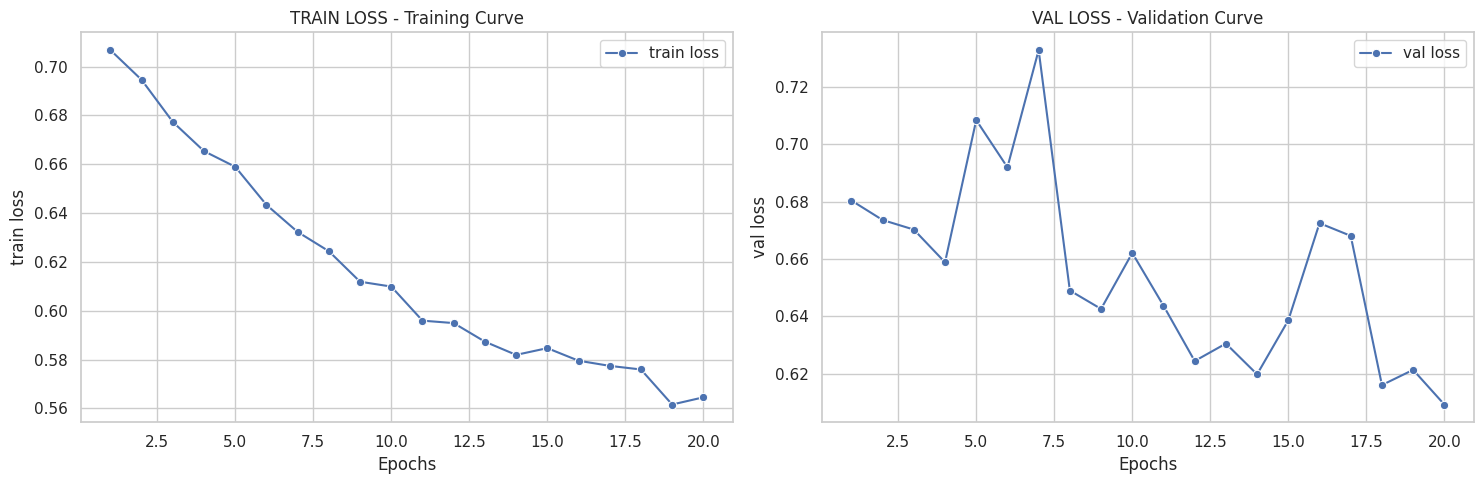
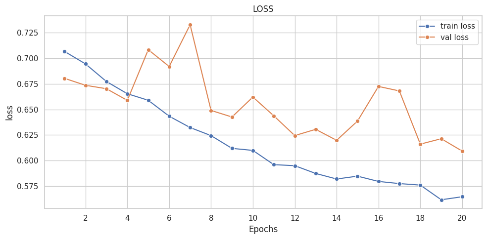
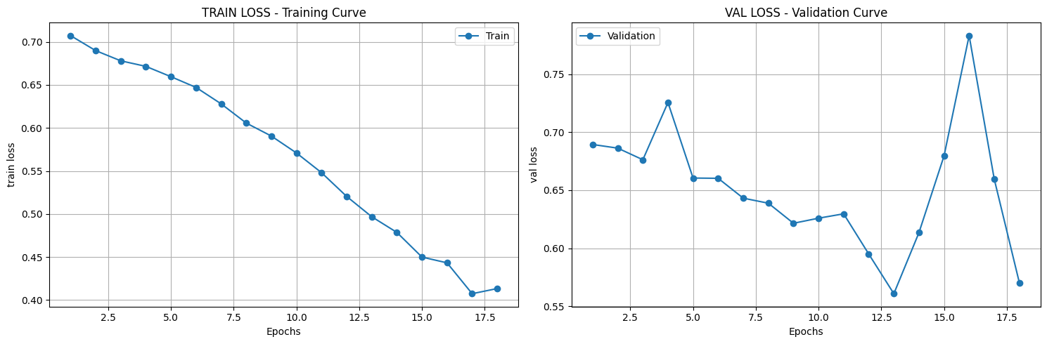
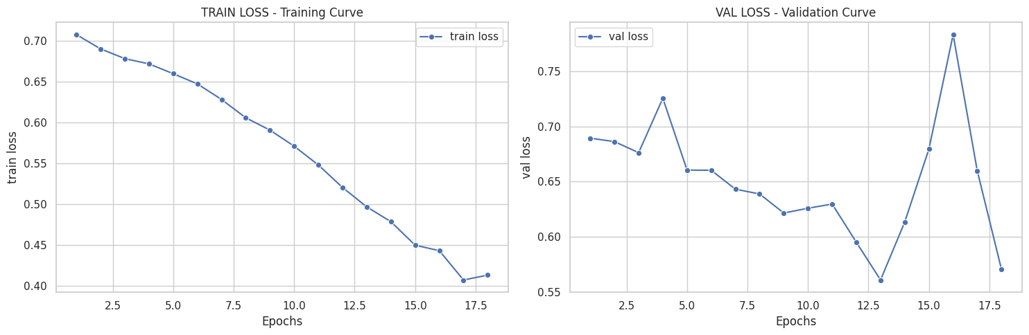
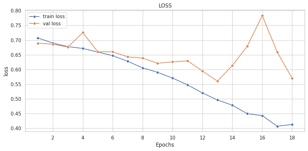
([{'val loss': 0.6803982134946843,
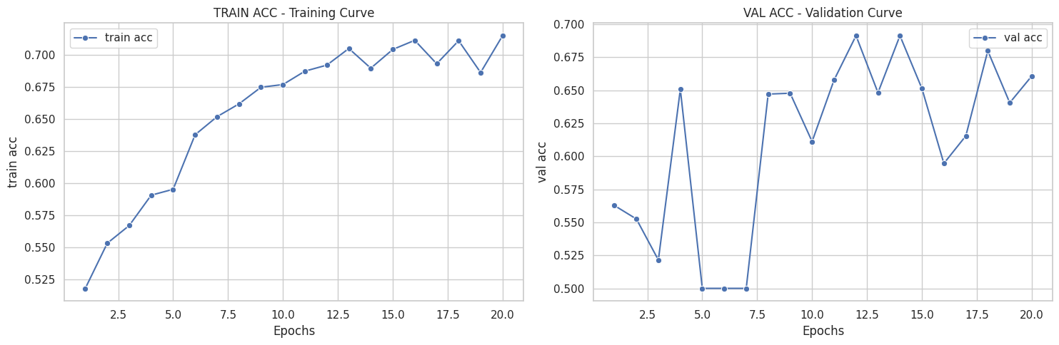
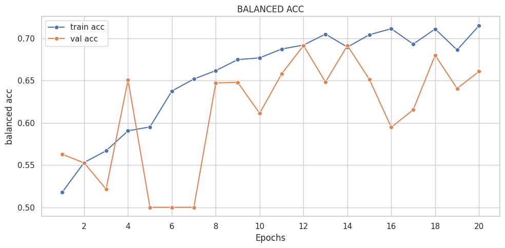
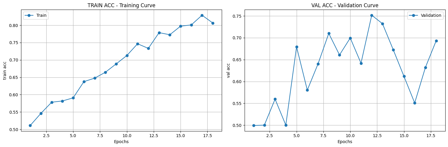
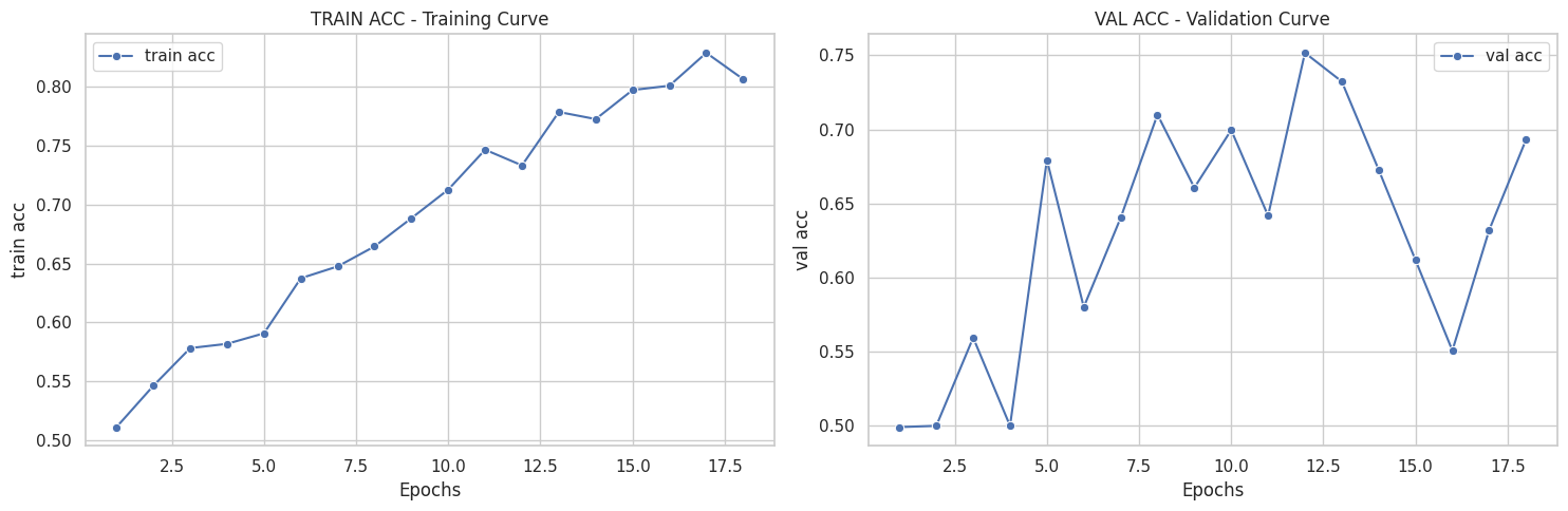
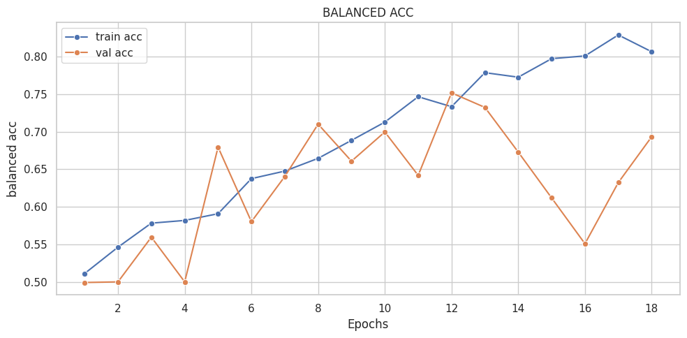
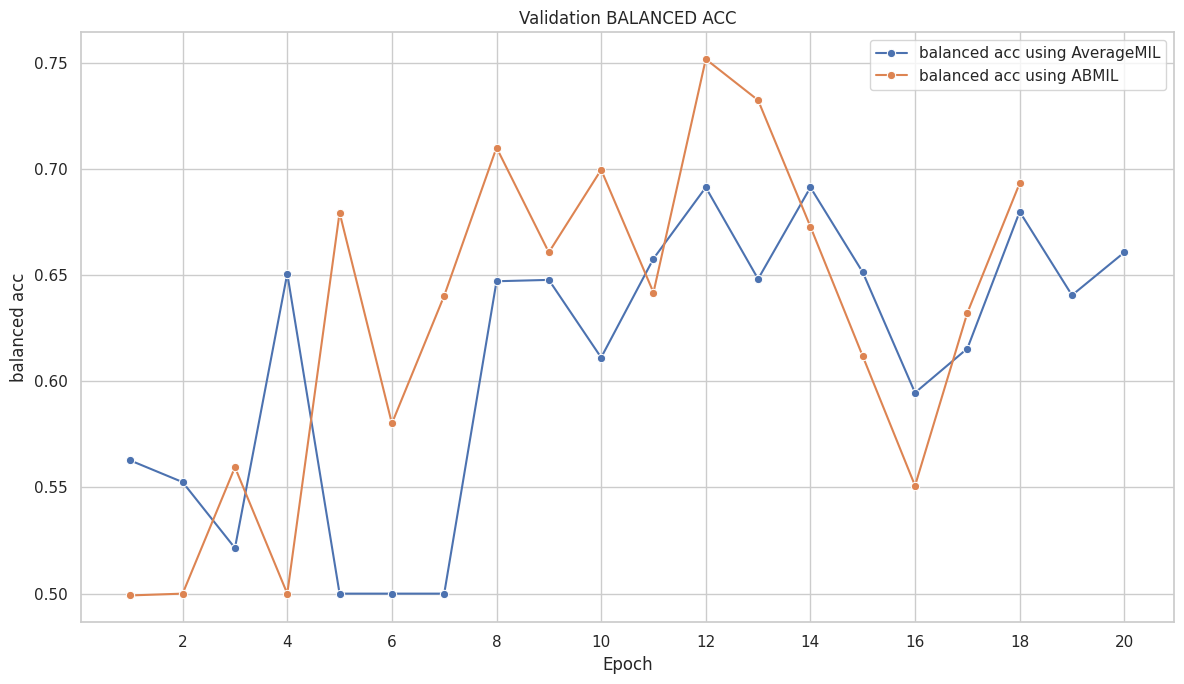
   'val acc': 0.5627125850340136,
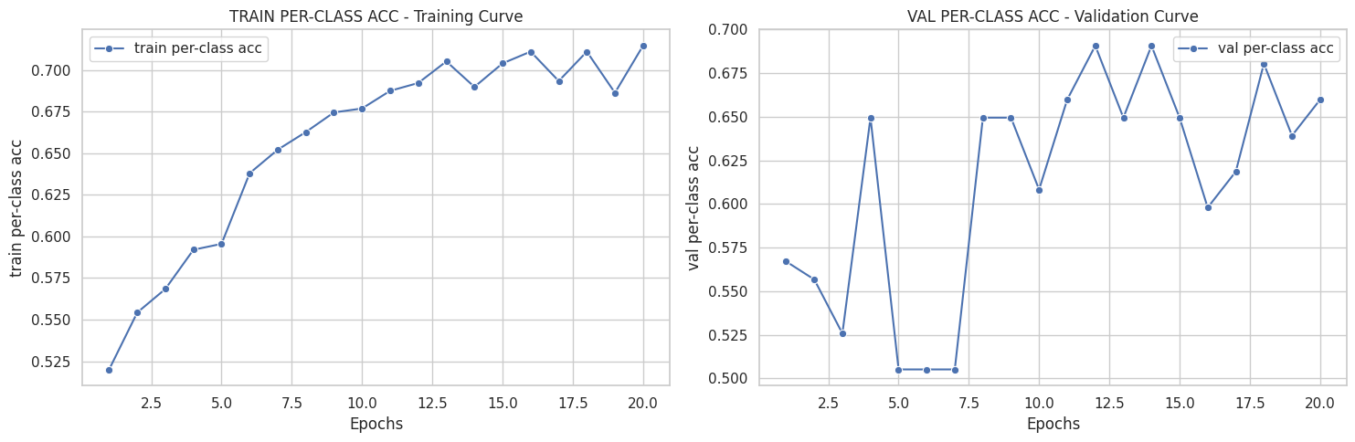
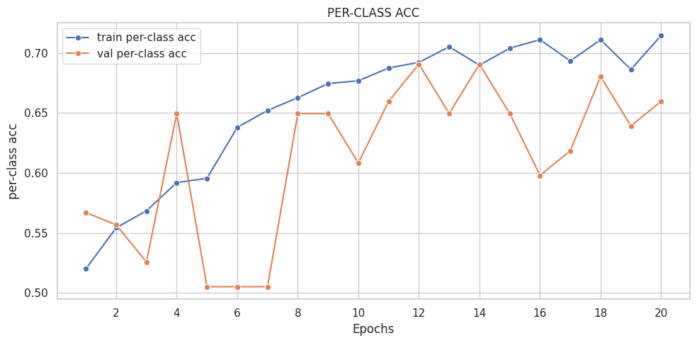
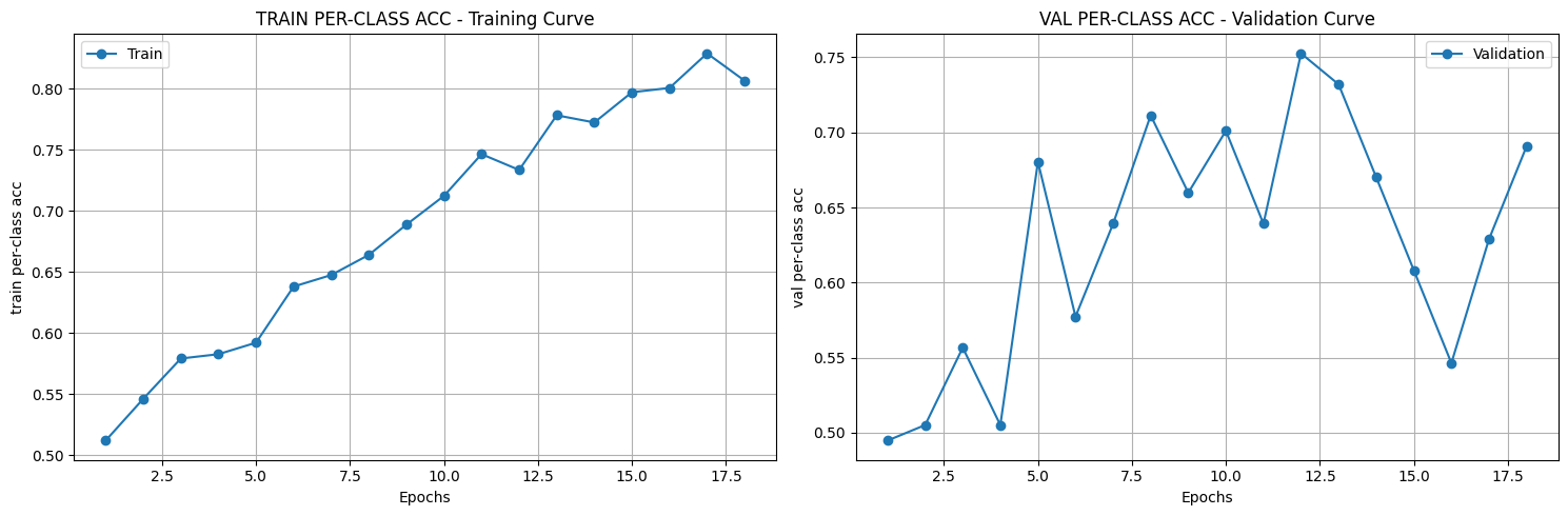
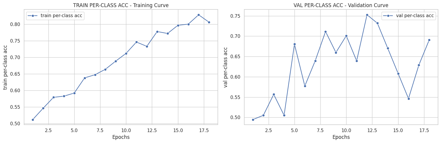
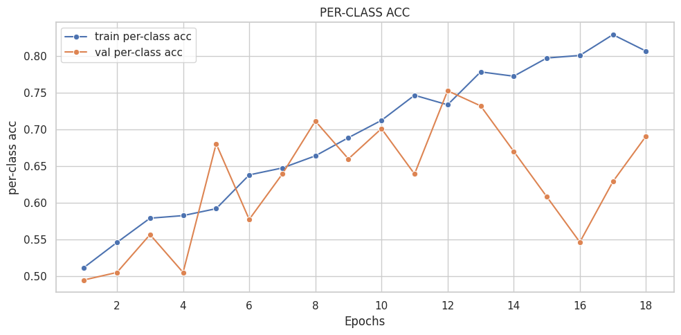
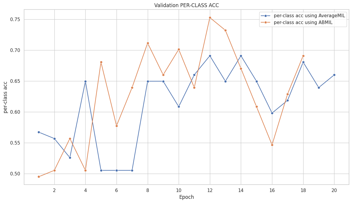
   'val per-class acc': 0.5670103092783505,
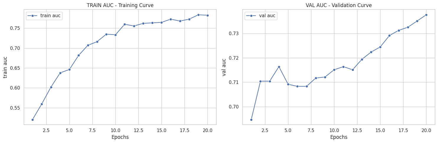
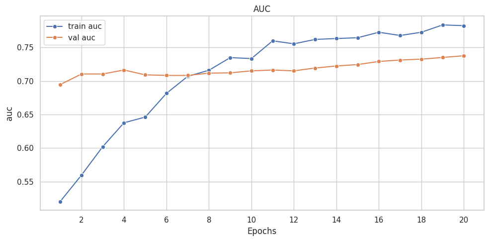
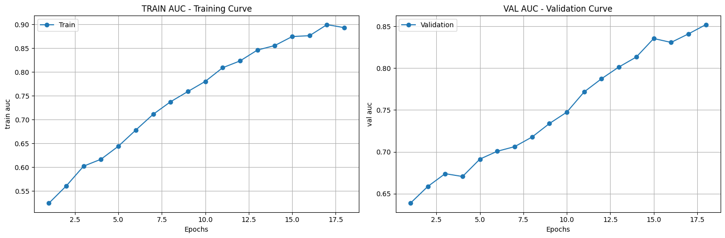
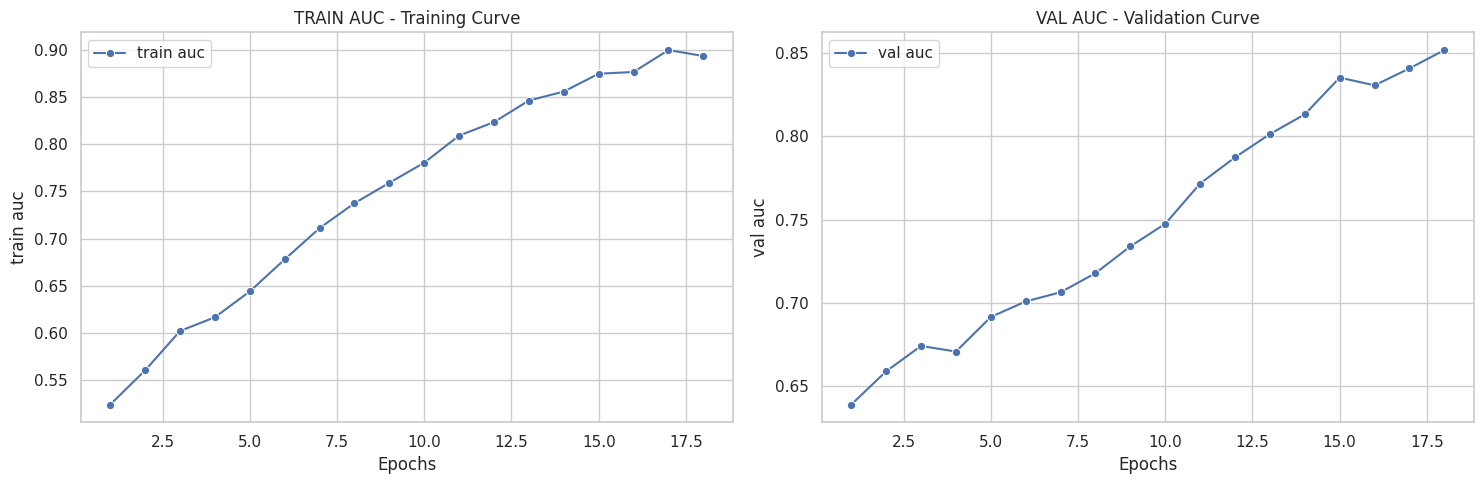
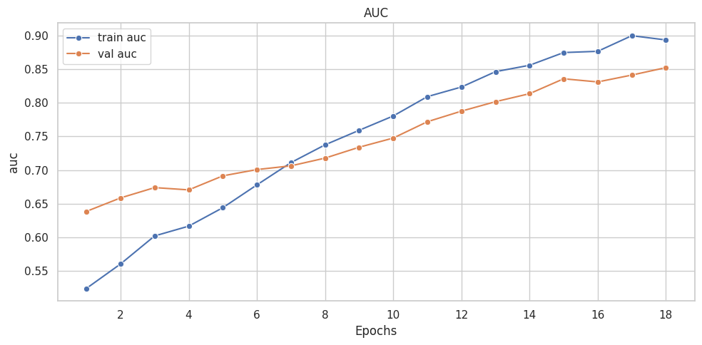
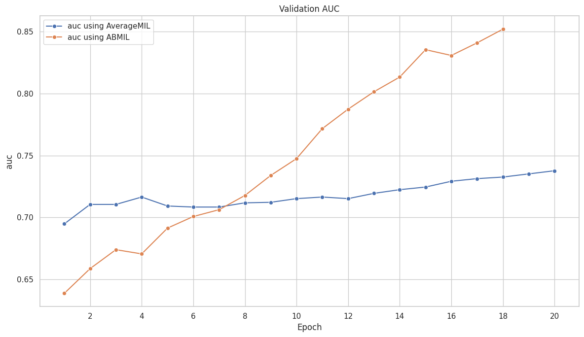
   'val auc': 0.6947278911564626},
  {'val loss': 0.6735972857352385,
   'val acc': 0.5525085034013605,
   'val per-class acc': 0.5567010309278351,
   'val auc': 0.7104591836734694},
  {'val loss': 0.6702608410845098,
   'val acc': 0.5214710884353742,
   'val per-class acc': 0.5257731958762887,
   'val auc': 0.7104591836734694},
  {'val loss': 0.658846736876006,
   'val acc': 0.6507227891156463,
   'val per-class acc': 0.6494845360824743,
   'val auc': 0.7164115646258503},
  {'val loss': 0.7084451502131432,
   'val acc': 0.5,
   'val per-class acc': 0.5051546391752577,
   'val auc': 0.7091836734693877},
  {'val loss': 0.6919781800705133,
   'val acc': 0.5,
   'val per-class acc': 0.5051546391752577,
   'val auc': 0.7083333333333335},
  {'val loss': 0.7328733577556217,
   'val acc': 0.5,
   'val per-class acc': 0.5051546391752577,
   'val auc': 0.7083333333333334},
  {'val loss': 0.6490099599066469,
   'val acc': 0.6471088435374149,
   'val per-class acc': 0.6494845360824743,
   'val auc': 0.7117346938775511},
  {'val loss': 0.6425867612214432,
   'val acc': 0.6477465986394558,
   'val per-class acc': 0.6494845360824743,
   'val auc': 0.7121598639455783},
  {'val loss': 0.6621069063230888,
   'val acc': 0.6111819727891157,
   'val per-class acc': 0.6082474226804123,
   'val auc': 0.7151360544217689},
  {'val loss': 0.6437243203219679,
   'val acc': 0.6577380952380952,
   'val per-class acc': 0.6597938144329897,
   'val auc': 0.7164115646258504},
  {'val loss': 0.6244144886732101,
   'val acc': 0.6913265306122449,
   'val per-class acc': 0.6907216494845361,
   'val auc': 0.7151360544217686},
  {'val loss': 0.6305080309663851,
   'val acc': 0.648171768707483,
   'val per-class acc': 0.6494845360824743,
   'val auc': 0.7193877551020408},
  {'val loss': 0.6197766895146714,
   'val acc': 0.6913265306122449,
   'val per-class acc': 0.6907216494845361,
   'val auc': 0.7223639455782312},
  {'val loss': 0.6386314140459926,
   'val acc': 0.6513605442176871,
   'val per-class acc': 0.6494845360824743,
   'val auc': 0.7244897959183674},
  {'val loss': 0.6724980127104779,
   'val acc': 0.5946003401360545,
   'val per-class acc': 0.5979381443298969,
   'val auc': 0.7291666666666667},
  {'val loss': 0.668074183780508,
   'val acc': 0.6154336734693877,
   'val per-class acc': 0.6185567010309279,
   'val auc': 0.7312925170068028},
  {'val loss': 0.6160321704198405,
   'val acc': 0.6798469387755102,
   'val per-class acc': 0.6804123711340206,
   'val auc': 0.7325680272108844},
  {'val loss': 0.6213401637433731,
   'val acc': 0.6405187074829932,
   'val per-class acc': 0.6391752577319587,
   'val auc': 0.7351190476190477},
  {'val loss': 0.6092413214524997,
   'val acc': 0.6607142857142857,
   'val per-class acc': 0.6597938144329897,
   'val auc': 0.7376700680272109}],
 [{'train loss': 0.7067322431413351,
   'train acc': 0.5178023873786137,
   'train per-class acc': 0.5200471698113207,
   'train auc': 0.5205153176215254},
  {'train loss': 0.6945402914623044,
   'train acc': 0.5529925707448733,
   'train per-class acc': 0.5542452830188679,
   'train auc': 0.5597651576282033},
  {'train loss': 0.677320071724507,
   'train acc': 0.5667992988118757,
   'train per-class acc': 0.5683962264150944,
   'train auc': 0.6021647792092156},
  {'train loss': 0.6653487175211029,
   'train acc': 0.5904449205598374,
   'train per-class acc': 0.5919811320754716,
   'train auc': 0.6377472940259885},
  {'train loss': 0.6589468236626038,
   'train acc': 0.5950610757116225,
   'train per-class acc': 0.5955188679245284,
   'train auc': 0.6462172013689863},
  {'train loss': 0.6433602210555999,
   'train acc': 0.6375831269651353,
   'train per-class acc': 0.6379716981132075,
   'train auc': 0.6815938117365536},
  {'train loss': 0.6322723758529942,
   'train acc': 0.6516903642282756,
   'train per-class acc': 0.652122641509434,
   'train auc': 0.7069144940037286},
  {'train loss': 0.6243803047065465,
   'train acc': 0.6616822949998609,
   'train per-class acc': 0.6627358490566038,
   'train auc': 0.7160410695901389},
  {'train loss': 0.6118933894794505,
   'train acc': 0.6746320153593589,
   'train per-class acc': 0.6745283018867925,
   'train auc': 0.7348618492445533},
  {'train loss': 0.6099064529627422,
   'train acc': 0.6767411447174378,
   'train per-class acc': 0.6768867924528302,
   'train auc': 0.7334372130554551},
  {'train loss': 0.5959538500316722,
   'train acc': 0.6871838392832299,
   'train per-class acc': 0.6875,
   'train auc': 0.7598875873007038},
  {'train loss': 0.594957460710814,
   'train acc': 0.6919029466596177,
   'train per-class acc': 0.6922169811320755,
   'train auc': 0.7554189042544311},
  {'train loss': 0.5873530111627056,
   'train acc': 0.7048554495116726,
   'train per-class acc': 0.7051886792452831,
   'train auc': 0.7619855866885555},
  {'train loss': 0.5819371846276071,
   'train acc': 0.6894933081054009,
   'train per-class acc': 0.6898584905660378,
   'train auc': 0.7633044881604942},
  {'train loss': 0.5847031294702077,
   'train acc': 0.704101394028771,
   'train per-class acc': 0.7040094339622641,
   'train auc': 0.7645176549152731},
  {'train loss': 0.5795527598732766,
   'train acc': 0.7112301399593756,
   'train per-class acc': 0.7110849056603774,
   'train auc': 0.772653663151451},
  {'train loss': 0.5774440601872245,
   'train acc': 0.6929575113386572,
   'train per-class acc': 0.6933962264150944,
   'train auc': 0.7678343860430173},
  {'train loss': 0.575963072298657,
   'train acc': 0.7109296307632377,
   'train per-class acc': 0.7110849056603774,
   'train auc': 0.772687053062133},
  {'train loss': 0.5616160210019926,
   'train acc': 0.6861292746041905,
   'train per-class acc': 0.6863207547169812,
   'train auc': 0.7835832939146888},
  {'train loss': 0.5645616454520386,
   'train acc': 0.7148445977907009,
   'train per-class acc': 0.714622641509434,
   'train auc': 0.7825036868026378}])
Code
# Sets the random seed (for reproducibility)
torch.manual_seed(2023)

# Get data loaders for train-val-test split evaluation
feats_dirpath, csv_fpath = './feats_pt/', './tcga_lung_splits.csv'
loader_kwargs = {'batch_size': 1, 'num_workers': 2, 'pin_memory': False} # Batch size set to 1 due to variable bag sizes. Hard to collate.
train_dataset, val_dataset, test_dataset = [MILDataset(feats_dirpath, csv_fpath, which_split=split) for split in ['train', 'val', 'test']]
train_loader = torch.utils.data.DataLoader(train_dataset, shuffle=True, **loader_kwargs)
val_loader = torch.utils.data.DataLoader(val_dataset, shuffle=False, **loader_kwargs)
test_loader = torch.utils.data.DataLoader(test_dataset, shuffle=False, **loader_kwargs)

# Get model, optimizer, and loss function
device = torch.device('cpu')
model = AverageMIL(input_dim=320, hidden_dim=64).to(device)
optimizer = torch.optim.AdamW(model.parameters(), lr=1e-4, weight_decay=1e-5)
loss_fn = nn.CrossEntropyLoss()

# Set-up train-validation loop and early stopping
num_epochs, min_early_stopping, patience, counter = 20, 10, 5, 0
lowest_val_loss, best_model = np.inf, None
all_train_logs_amil, all_val_logs_amil = [], [] # TODO: do something with train_log / val_log every epoch to help visualize performance curves?
for epoch in range(num_epochs):
    train_log = traineval_epoch(epoch, model, train_loader, optimizer=optimizer, split='train', device=device, verbose=2, print_every=200)
    val_log = traineval_epoch(epoch, model, val_loader, optimizer=None, split='val', device=device, verbose=1)
    val_loss = val_log['val loss']
    # Append train and validation logs for visualization
    all_train_logs_amil.append(train_log)
    all_val_logs_amil.append(val_log)
    # Early stopping: If validation loss does not go down for <patience> epochs after <min_early_stopping> epochs, stop model training early
    if (epoch > min_early_stopping):
        if (val_loss < lowest_val_loss):
            print(f'Resetting early-stopping counter: {lowest_val_loss:.04f} -> {val_loss:.04f}...')
            lowest_val_loss, counter, best_model = val_loss, 0, copy.deepcopy(model)
        else:
            print(f'Early-stopping counter updating: {counter}/{patience} -> {counter+1}/{patience}...')
            counter += 1

    if counter >= patience: break
    print()

# Report best model (lowest validation loss) on test split
best_model = model if (best_model is None) else best_model
test_log = traineval_epoch(epoch, best_model, test_loader, optimizer=None, split='test', device=device, verbose=1)

# TODO: visualizing train and validation performance curves for AverageMIL
Epoch 0:     Batch 199   Avg Loss: 0.7137    Label: 1    Bag Size: 957
Epoch 0:     Batch 399   Avg Loss: 0.7084    Label: 1    Bag Size: 1131
Epoch 0:     Batch 599   Avg Loss: 0.7093    Label: 1    Bag Size: 1342
Epoch 0:     Batch 799   Avg Loss: 0.7075    Label: 1    Bag Size: 2319
### (Train Summary) ###
Epoch 0:    Train loss: 0.7067   Train acc: 0.5178  Train per-class acc: 0.5200  Train auc: 0.5205
### (Val Summary) ###
Epoch 0:      Val loss: 0.6804     Val acc: 0.5627  Val per-class acc: 0.5670      Val auc: 0.6947

Epoch 1:     Batch 199   Avg Loss: 0.6892    Label: 1    Bag Size: 2830
Epoch 1:     Batch 399   Avg Loss: 0.6933    Label: 0    Bag Size: 4905
Epoch 1:     Batch 599   Avg Loss: 0.6951    Label: 0    Bag Size: 5624
Epoch 1:     Batch 799   Avg Loss: 0.6919    Label: 0    Bag Size: 1298
### (Train Summary) ###
Epoch 1:    Train loss: 0.6945   Train acc: 0.5530  Train per-class acc: 0.5542  Train auc: 0.5598
### (Val Summary) ###
Epoch 1:      Val loss: 0.6736     Val acc: 0.5525  Val per-class acc: 0.5567      Val auc: 0.7105

Epoch 2:     Batch 199   Avg Loss: 0.6910    Label: 0    Bag Size: 3509
Epoch 2:     Batch 399   Avg Loss: 0.6808    Label: 0    Bag Size: 6975
Epoch 2:     Batch 599   Avg Loss: 0.6799    Label: 0    Bag Size: 1555
Epoch 2:     Batch 799   Avg Loss: 0.6784    Label: 0    Bag Size: 4302
### (Train Summary) ###
Epoch 2:    Train loss: 0.6773   Train acc: 0.5668  Train per-class acc: 0.5684  Train auc: 0.6022
### (Val Summary) ###
Epoch 2:      Val loss: 0.6703     Val acc: 0.5215  Val per-class acc: 0.5258      Val auc: 0.7105

Epoch 3:     Batch 199   Avg Loss: 0.6628    Label: 0    Bag Size: 6237
Epoch 3:     Batch 399   Avg Loss: 0.6645    Label: 0    Bag Size: 6577
Epoch 3:     Batch 599   Avg Loss: 0.6679    Label: 1    Bag Size: 223
Epoch 3:     Batch 799   Avg Loss: 0.6640    Label: 0    Bag Size: 3368
### (Train Summary) ###
Epoch 3:    Train loss: 0.6653   Train acc: 0.5904  Train per-class acc: 0.5920  Train auc: 0.6377
### (Val Summary) ###
Epoch 3:      Val loss: 0.6588     Val acc: 0.6507  Val per-class acc: 0.6495      Val auc: 0.7164

Epoch 4:     Batch 199   Avg Loss: 0.6642    Label: 1    Bag Size: 1563
Epoch 4:     Batch 399   Avg Loss: 0.6751    Label: 0    Bag Size: 1512
Epoch 4:     Batch 599   Avg Loss: 0.6637    Label: 1    Bag Size: 8248
Epoch 4:     Batch 799   Avg Loss: 0.6586    Label: 1    Bag Size: 933
### (Train Summary) ###
Epoch 4:    Train loss: 0.6589   Train acc: 0.5951  Train per-class acc: 0.5955  Train auc: 0.6462
### (Val Summary) ###
Epoch 4:      Val loss: 0.7084     Val acc: 0.5000  Val per-class acc: 0.5052      Val auc: 0.7092

Epoch 5:     Batch 199   Avg Loss: 0.6623    Label: 0    Bag Size: 377
Epoch 5:     Batch 399   Avg Loss: 0.6632    Label: 0    Bag Size: 1856
Epoch 5:     Batch 599   Avg Loss: 0.6511    Label: 1    Bag Size: 3239
Epoch 5:     Batch 799   Avg Loss: 0.6467    Label: 0    Bag Size: 356
### (Train Summary) ###
Epoch 5:    Train loss: 0.6434   Train acc: 0.6376  Train per-class acc: 0.6380  Train auc: 0.6816
### (Val Summary) ###
Epoch 5:      Val loss: 0.6920     Val acc: 0.5000  Val per-class acc: 0.5052      Val auc: 0.7083

Epoch 6:     Batch 199   Avg Loss: 0.6496    Label: 1    Bag Size: 4575
Epoch 6:     Batch 399   Avg Loss: 0.6349    Label: 1    Bag Size: 4743
Epoch 6:     Batch 599   Avg Loss: 0.6316    Label: 0    Bag Size: 4420
Epoch 6:     Batch 799   Avg Loss: 0.6311    Label: 1    Bag Size: 4480
### (Train Summary) ###
Epoch 6:    Train loss: 0.6323   Train acc: 0.6517  Train per-class acc: 0.6521  Train auc: 0.7069
### (Val Summary) ###
Epoch 6:      Val loss: 0.7329     Val acc: 0.5000  Val per-class acc: 0.5052      Val auc: 0.7083

Epoch 7:     Batch 199   Avg Loss: 0.6297    Label: 0    Bag Size: 4443
Epoch 7:     Batch 399   Avg Loss: 0.6245    Label: 1    Bag Size: 1261
Epoch 7:     Batch 599   Avg Loss: 0.6233    Label: 1    Bag Size: 4893
Epoch 7:     Batch 799   Avg Loss: 0.6258    Label: 1    Bag Size: 5530
### (Train Summary) ###
Epoch 7:    Train loss: 0.6244   Train acc: 0.6617  Train per-class acc: 0.6627  Train auc: 0.7160
### (Val Summary) ###
Epoch 7:      Val loss: 0.6490     Val acc: 0.6471  Val per-class acc: 0.6495      Val auc: 0.7117

Epoch 8:     Batch 199   Avg Loss: 0.6155    Label: 1    Bag Size: 5553
Epoch 8:     Batch 399   Avg Loss: 0.6293    Label: 0    Bag Size: 8315
Epoch 8:     Batch 599   Avg Loss: 0.6184    Label: 0    Bag Size: 4905
Epoch 8:     Batch 799   Avg Loss: 0.6141    Label: 1    Bag Size: 3630
### (Train Summary) ###
Epoch 8:    Train loss: 0.6119   Train acc: 0.6746  Train per-class acc: 0.6745  Train auc: 0.7349
### (Val Summary) ###
Epoch 8:      Val loss: 0.6426     Val acc: 0.6477  Val per-class acc: 0.6495      Val auc: 0.7122

Epoch 9:     Batch 199   Avg Loss: 0.6157    Label: 0    Bag Size: 2482
Epoch 9:     Batch 399   Avg Loss: 0.6002    Label: 0    Bag Size: 1856
Epoch 9:     Batch 599   Avg Loss: 0.6062    Label: 0    Bag Size: 384
Epoch 9:     Batch 799   Avg Loss: 0.6094    Label: 0    Bag Size: 579
### (Train Summary) ###
Epoch 9:    Train loss: 0.6099   Train acc: 0.6767  Train per-class acc: 0.6769  Train auc: 0.7334
### (Val Summary) ###
Epoch 9:      Val loss: 0.6621     Val acc: 0.6112  Val per-class acc: 0.6082      Val auc: 0.7151

Epoch 10:    Batch 199   Avg Loss: 0.5707    Label: 1    Bag Size: 3912
Epoch 10:    Batch 399   Avg Loss: 0.6012    Label: 0    Bag Size: 6484
Epoch 10:    Batch 599   Avg Loss: 0.6039    Label: 1    Bag Size: 3609
Epoch 10:    Batch 799   Avg Loss: 0.5971    Label: 0    Bag Size: 345
### (Train Summary) ###
Epoch 10:   Train loss: 0.5960   Train acc: 0.6872  Train per-class acc: 0.6875  Train auc: 0.7599
### (Val Summary) ###
Epoch 10:     Val loss: 0.6437     Val acc: 0.6577  Val per-class acc: 0.6598      Val auc: 0.7164

Epoch 11:    Batch 199   Avg Loss: 0.5891    Label: 0    Bag Size: 1329
Epoch 11:    Batch 399   Avg Loss: 0.6048    Label: 0    Bag Size: 3423
Epoch 11:    Batch 599   Avg Loss: 0.5980    Label: 1    Bag Size: 5204
Epoch 11:    Batch 799   Avg Loss: 0.5910    Label: 1    Bag Size: 1342
### (Train Summary) ###
Epoch 11:   Train loss: 0.5950   Train acc: 0.6919  Train per-class acc: 0.6922  Train auc: 0.7554
### (Val Summary) ###
Epoch 11:     Val loss: 0.6244     Val acc: 0.6913  Val per-class acc: 0.6907      Val auc: 0.7151
Resetting early-stopping counter: inf -> 0.6244...

Epoch 12:    Batch 199   Avg Loss: 0.5887    Label: 1    Bag Size: 5400
Epoch 12:    Batch 399   Avg Loss: 0.5753    Label: 0    Bag Size: 6074
Epoch 12:    Batch 599   Avg Loss: 0.5857    Label: 0    Bag Size: 4085
Epoch 12:    Batch 799   Avg Loss: 0.5852    Label: 0    Bag Size: 2415
### (Train Summary) ###
Epoch 12:   Train loss: 0.5874   Train acc: 0.7049  Train per-class acc: 0.7052  Train auc: 0.7620
### (Val Summary) ###
Epoch 12:     Val loss: 0.6305     Val acc: 0.6482  Val per-class acc: 0.6495      Val auc: 0.7194
Early-stopping counter updating: 0/5 -> 1/5...

Epoch 13:    Batch 199   Avg Loss: 0.5654    Label: 0    Bag Size: 4486
Epoch 13:    Batch 399   Avg Loss: 0.5794    Label: 0    Bag Size: 464
Epoch 13:    Batch 599   Avg Loss: 0.5889    Label: 0    Bag Size: 8841
Epoch 13:    Batch 799   Avg Loss: 0.5794    Label: 0    Bag Size: 1334
### (Train Summary) ###
Epoch 13:   Train loss: 0.5819   Train acc: 0.6895  Train per-class acc: 0.6899  Train auc: 0.7633
### (Val Summary) ###
Epoch 13:     Val loss: 0.6198     Val acc: 0.6913  Val per-class acc: 0.6907      Val auc: 0.7224
Resetting early-stopping counter: 0.6244 -> 0.6198...

Epoch 14:    Batch 199   Avg Loss: 0.5543    Label: 0    Bag Size: 2093
Epoch 14:    Batch 399   Avg Loss: 0.5704    Label: 0    Bag Size: 9103
Epoch 14:    Batch 599   Avg Loss: 0.5775    Label: 1    Bag Size: 2906
Epoch 14:    Batch 799   Avg Loss: 0.5823    Label: 1    Bag Size: 1805
### (Train Summary) ###
Epoch 14:   Train loss: 0.5847   Train acc: 0.7041  Train per-class acc: 0.7040  Train auc: 0.7645
### (Val Summary) ###
Epoch 14:     Val loss: 0.6386     Val acc: 0.6514  Val per-class acc: 0.6495      Val auc: 0.7245
Early-stopping counter updating: 0/5 -> 1/5...

Epoch 15:    Batch 199   Avg Loss: 0.5708    Label: 1    Bag Size: 711
Epoch 15:    Batch 399   Avg Loss: 0.5638    Label: 1    Bag Size: 980
Epoch 15:    Batch 599   Avg Loss: 0.5857    Label: 0    Bag Size: 3167
Epoch 15:    Batch 799   Avg Loss: 0.5807    Label: 1    Bag Size: 5346
### (Train Summary) ###
Epoch 15:   Train loss: 0.5796   Train acc: 0.7112  Train per-class acc: 0.7111  Train auc: 0.7727
### (Val Summary) ###
Epoch 15:     Val loss: 0.6725     Val acc: 0.5946  Val per-class acc: 0.5979      Val auc: 0.7292
Early-stopping counter updating: 1/5 -> 2/5...

Epoch 16:    Batch 199   Avg Loss: 0.5944    Label: 0    Bag Size: 4156
Epoch 16:    Batch 399   Avg Loss: 0.5885    Label: 1    Bag Size: 2068
Epoch 16:    Batch 599   Avg Loss: 0.5782    Label: 1    Bag Size: 3720
Epoch 16:    Batch 799   Avg Loss: 0.5760    Label: 1    Bag Size: 6535
### (Train Summary) ###
Epoch 16:   Train loss: 0.5774   Train acc: 0.6930  Train per-class acc: 0.6934  Train auc: 0.7678
### (Val Summary) ###
Epoch 16:     Val loss: 0.6681     Val acc: 0.6154  Val per-class acc: 0.6186      Val auc: 0.7313
Early-stopping counter updating: 2/5 -> 3/5...

Epoch 17:    Batch 199   Avg Loss: 0.6217    Label: 1    Bag Size: 1594
Epoch 17:    Batch 399   Avg Loss: 0.6043    Label: 1    Bag Size: 5042
Epoch 17:    Batch 599   Avg Loss: 0.5980    Label: 1    Bag Size: 4271
Epoch 17:    Batch 799   Avg Loss: 0.5737    Label: 0    Bag Size: 3418
### (Train Summary) ###
Epoch 17:   Train loss: 0.5760   Train acc: 0.7109  Train per-class acc: 0.7111  Train auc: 0.7727
### (Val Summary) ###
Epoch 17:     Val loss: 0.6160     Val acc: 0.6798  Val per-class acc: 0.6804      Val auc: 0.7326
Resetting early-stopping counter: 0.6198 -> 0.6160...

Epoch 18:    Batch 199   Avg Loss: 0.5474    Label: 0    Bag Size: 2924
Epoch 18:    Batch 399   Avg Loss: 0.5506    Label: 0    Bag Size: 5320
Epoch 18:    Batch 599   Avg Loss: 0.5532    Label: 0    Bag Size: 2522
Epoch 18:    Batch 799   Avg Loss: 0.5585    Label: 0    Bag Size: 446
### (Train Summary) ###
Epoch 18:   Train loss: 0.5616   Train acc: 0.6861  Train per-class acc: 0.6863  Train auc: 0.7836
### (Val Summary) ###
Epoch 18:     Val loss: 0.6213     Val acc: 0.6405  Val per-class acc: 0.6392      Val auc: 0.7351
Early-stopping counter updating: 0/5 -> 1/5...

Epoch 19:    Batch 199   Avg Loss: 0.5784    Label: 1    Bag Size: 1063
Epoch 19:    Batch 399   Avg Loss: 0.5670    Label: 1    Bag Size: 3959
Epoch 19:    Batch 599   Avg Loss: 0.5662    Label: 0    Bag Size: 1455
Epoch 19:    Batch 799   Avg Loss: 0.5631    Label: 0    Bag Size: 4642
### (Train Summary) ###
Epoch 19:   Train loss: 0.5646   Train acc: 0.7148  Train per-class acc: 0.7146  Train auc: 0.7825
### (Val Summary) ###
Epoch 19:     Val loss: 0.6092     Val acc: 0.6607  Val per-class acc: 0.6598      Val auc: 0.7377
Resetting early-stopping counter: 0.6160 -> 0.6092...

### (Test Summary) ###
Epoch 19:    Test loss: 0.5561    Test acc: 0.6837  Test per-class acc: 0.6837    Test auc: 0.8401
Code
import seaborn as sns
import matplotlib.pyplot as plt

# TODO: visualizing train and validation performance curves for AverageMIL
epochs = range(1, len(all_train_logs_amil) + 1)  # Assuming each log contains data for one epoch

for metric1, metric2 in zip(all_train_logs_amil[0].keys(), all_val_logs_amil[0].keys()) :
    if metric1.startswith('train') or metric2.startswith('val'):
        train_metric_amil = [log[metric1] for log in all_train_logs_amil]
        val_metric_amil = [log[metric2] for log in all_val_logs_amil]

        # Set Seaborn style
        sns.set(style="whitegrid")

        # Create a figure and axis object
        fig, axes = plt.subplots(nrows=1, ncols=2, figsize=(15, 5))

        # Plot train curve with Seaborn
        sns.lineplot(x=epochs, y=train_metric_amil, ax=axes[0], marker='o', label=metric1)
        axes[0].set_xlabel('Epochs')
        axes[0].set_ylabel(metric1)
        axes[0].set_title(f'{metric1.upper()} - Training Curve')

        # Plot validation curve with Seaborn
        sns.lineplot(x=epochs, y=val_metric_amil, ax=axes[1], marker='o', label=metric2)
        axes[1].set_xlabel('Epochs')
        axes[1].set_ylabel(metric2)
        axes[1].set_title(f'{metric2.upper()} - Validation Curve')
        #fig.savefig(f'{metric1.upper()}_AverageMIL.png', dpi=300)
        # Adjust layout
        plt.tight_layout()
        plt.show()

Code
# TODO: visualizing train and validation performance curves for AverageMIL
epochs = range(1, len(all_train_logs_amil) + 1)  # Assuming each log contains data for one epoch
label = ['loss', 'balanced acc','per-class acc', 'auc']
counter = 0
for metric1, metric2 in zip(all_train_logs_amil[0].keys(), all_val_logs_amil[0].keys()) :
    if metric1.startswith('train') or metric2.startswith('val'):
        train_metric_amil = [log[metric1] for log in all_train_logs_amil]
        val_metric_amil = [log[metric2] for log in all_val_logs_amil]
        # Create a figure and axis object
        fig, ax = plt.subplots(figsize=(10, 5))

        # Plot train and validation curves on the same plot
        sns.lineplot(x=epochs, y=train_metric_amil, ax=ax, marker='o', label=metric1)
        sns.lineplot(x=epochs, y=val_metric_amil, ax=ax, marker='o', label=metric2)
        ax.set_xticks(range(2, len(train_metric_amil)+2, 2))
        ax.set_xlabel('Epochs')
        ax.set_ylabel(label[counter])
        ax.set_title(f'{label[counter].upper()}')

        # Adjust layout
        plt.tight_layout()

        # Save the figure
        fig.savefig(f'{metric1.upper()}_AMIL.png', dpi=300)
        counter +=1
        # Show the plot
        plt.show()

Question 2. Implement Attention-Based Multiple Instance Learning (ABMIL) (15 points)

Following your experimentation with AverageMIL, you are ready to implement a more sophisticated model for LUAD vs. LUSC subtyping. Formally, let \(\mathbf{H}=\left\{\mathbf{h}_1, \ldots, \mathbf{h}_M\right\} \in \mathbb{R}^{M \times D}\) be a bag of \(M\) patch embeddings, with each embedding having dimension size \(D\). Ilse et al. 2018 proposed the following attention-based MIL pooling operation:

\[ \mathbf{z} =\sum_{i=1}^M a_i \mathbf{h}_i, \quad \text{where} \enspace a_i=\frac{\exp \left\{\mathbf{w}^{\top}\left(\tanh \left(\mathbf{V h}_{i} ^ { \top }\right) \odot \operatorname{sigm}\left(\mathbf{U h}_i^{\top}\right)\right)\right\}}{\sum_{j=1}^M \exp \left\{\mathbf{w}^{\top}\left(\tanh \left(\mathbf{V} \mathbf{h}_j^{\top}\right) \odot \operatorname{sigm}\left(\mathbf{U h}_j^{\top}\right)\right)\right\}} \]

where \(\mathbf{w} \in \mathbb{R}^{L \times 1}\), \(\mathbf{V} \in \mathbb{R}^{L \times D}\), and \(\mathbf{U} \in \mathbb{R}^{L \times D}\) are learnable neural network parameters (implemented as fully-connected layers), and \(\mathbf{z} \in \mathbb{R}^{D}\) is the weighted average of all patch embeddings in \(\mathbf{H}\). The hyperbolic tangent \(\tanh (\cdot)\) element-wise non-linearity and sigmoid non-linearity are utilized for proper gradient flow.

Via PyTorch, the mathematical expression for computing \(a_m\) is implemented as the torch.nn module Attention_TanhSigmoidGating, which we use as a layer in ABMIL for calculating the weighted average of patch embeddings. The Colab Notebook provides an almost-ready implementation of ABMIL, with the forward pass implementation left incomplete in the ABMIL model definition.

  1. Finish implementing ABMIL via filling in the TODO section (in the forward pass section) of the ABMIL model definition.
  2. Report the balanced accuracy and overall AUC on the test split (answers are deterministic due to setting manual seed).
  3. Similar to AverageMIL, visualize the train and validation performance for the loss, balanced accuracy, per-class accuracy, and overall AUC metrics for 20 epochs (or until early stopping).
Code
class Attention_TanhSigmoidGating(nn.Module):
    def __init__(self, D=64, L=64, dropout=0.25):
        r"""
        Global attention pooling layer with tanh non-linearity and sigmoid gating (Ilse et al. 2018).

        Args:
            D (int): input feature dimension.
            L (int): hidden layer dimension. Notation changed from M from Ilse et al 2018, as M is overloaded to also describe # of patch embeddings in a WSI.
            dropout (float): Dropout probability.

        Returns:
            A_norm (torch.Tensor): [M x 1]-dim tensor of normalized attention scores (sum to 1)
        """
        super(Attention_TanhSigmoidGating, self).__init__()
        self.tanhV = nn.Sequential(*[nn.Linear(D, L), nn.Tanh(), nn.Dropout(dropout)])
        self.sigmU = nn.Sequential(*[nn.Linear(D, L), nn.Sigmoid(), nn.Dropout(dropout)])
        self.w = nn.Linear(L, 1)

    def forward(self, H):
        A_raw = self.w(self.tanhV(H).mul(self.sigmU(H))) # exponent term
        A_norm = F.softmax(A_raw, dim=0)                 # apply softmax to normalize weights to 1
        assert abs(A_norm.sum() - 1) < 1e-3              # Assert statement to check sum(A) ~= 1
        return A_norm


class ABMIL(nn.Module):
    def __init__(self, input_dim=320, hidden_dim=64, dropout=0.25, n_classes=2):
        r"""
        Attention-Based Multiple Instance Learning (Ilse et al. 2018).

        Args:
            input_dim (int): input feature dimension.
            hidden_dim (int): hidden layer dimension.
            dropout (float): Dropout probability.
            n_classes (int): Number of classes.
        """
        super(ABMIL, self).__init__()
        self.inst_level_fc = nn.Sequential(*[nn.Linear(input_dim, hidden_dim), nn.ReLU(), nn.Dropout(dropout)]) # Fully-Connected Layer, applied "instance-wise" to each embedding
        self.global_attn = Attention_TanhSigmoidGating(L=hidden_dim, D=hidden_dim)                              # Attention Function
        self.bag_level_classifier = nn.Linear(hidden_dim, n_classes)                                            # Bag-Level Classifier

    def forward(self, X: torch.randn(100, 320)):
        r"""
        Takes as input a [M x D]-dim bag of patch features (representing a WSI), and outputs: 1) logits for classification, 2) un-normalized attention scores.

        Args:
            X (torch.Tensor): [M x D]-dim bag of patch features (representing a WSI)

        Returns:
            logits (torch.Tensor): [1 x n_classes]-dim tensor of un-normalized logits for classification task.
            A_norm (torch.Tensor): [M,]- or [M x 1]-dim tensor of attention scores.
        """
        H_inst = self.inst_level_fc(X)        # TODO: 1. Process each feature embedding to be of size "hidden-dim"
        A_norm = self.global_attn(H_inst)        # TODO: 2. Get normalized attention scores for each embedding (s.t. sum(A_norm) ~= 1)
        z = (A_norm * H_inst).sum(dim=0).unsqueeze(0) # TODO: 3. Output of global attention pooling over the bag
        logits = self.bag_level_classifier(z)        # TODO: 4. Get un-normalized logits for classification task
        try:
            assert logits.shape == (1,2)
        except:
            print(f"Logit tensor shape is not formatted correctly. Should output [1 x 2] shape, but got {logits.shape} shape")
        return logits, A_norm
Code
# TODO: this cell requires a valid implementation of ABMIL first, and may not run. Largely copy-pasted from above cell.

# Sets the random seed (for reproducibility)
torch.manual_seed(2023)

# Get data loaders for train-val-test split evaluation
feats_dirpath, csv_fpath = './feats_pt/', './tcga_lung_splits.csv'
display(pd.read_csv(csv_fpath).head(10)) # visualize data
loader_kwargs = {'batch_size': 1, 'num_workers': 2, 'pin_memory': False} # Batch size set to 1 due to variable bag sizes. Hard to collate.
train_dataset, val_dataset, test_dataset = [MILDataset(feats_dirpath, csv_fpath, which_split=split) for split in ['train', 'val', 'test']]
train_loader = torch.utils.data.DataLoader(train_dataset, shuffle=True, **loader_kwargs)
val_loader = torch.utils.data.DataLoader(val_dataset, shuffle=False, **loader_kwargs)
test_loader = torch.utils.data.DataLoader(test_dataset, shuffle=False, **loader_kwargs)

# Get model, optimizer, and loss function
device = torch.device('cpu')
model = ABMIL(input_dim=320, hidden_dim=64).to(device)
optimizer = torch.optim.AdamW(model.parameters(), lr=1e-4, weight_decay=1e-5)
loss_fn = nn.CrossEntropyLoss()

# Set-up train-validation loop and early stopping
num_epochs, min_early_stopping, patience, counter = 20, 10, 5, 0
lowest_val_loss, best_model = np.inf, None
all_train_logs, all_val_logs = [], [] # TODO: do something with train_log / val_log every epoch to help visualize performance curves?
for epoch in range(num_epochs):
    train_log = traineval_epoch(epoch, model, train_loader, optimizer=optimizer, split='train', device=device, verbose=2, print_every=200)
    val_log = traineval_epoch(epoch, model, val_loader, optimizer=None, split='val', device=device, verbose=1)
    val_loss = val_log['val loss']
    # Append train and validation logs for visualization
    all_train_logs.append(train_log)
    all_val_logs.append(val_log)

    # Early stopping: If validation loss does not go down for <patience> epochs after <min_early_stopping> epochs, stop model training early
    if (epoch > min_early_stopping):
        if (val_loss < lowest_val_loss):
            print(f'Resetting early-stopping counter: {lowest_val_loss:.04f} -> {val_loss:.04f}...')
            lowest_val_loss, counter, best_model = val_loss, 0, copy.deepcopy(model)
        else:
            print(f'Early-stopping counter updating: {counter}/{patience} -> {counter+1}/{patience}...')
            counter += 1

    if counter >= patience: break
    print()

# Report best model (lowest validation loss) on test split
best_model = model if (best_model is None) else best_model
test_log = traineval_epoch(epoch, best_model, test_loader, optimizer=None, split='test', device=device, verbose=1)

# TODO: visualizing train and validation performance for ABMIL
case_id slide_id tumor_type OncoTreeSiteCode main_cancer_type sex project_id Diagnosis OncoTreeCode OncoTreeCode_Binarized split
0 TCGA-73-4676 TCGA-73-4676-01Z-00-DX1.4d781bbc-a45e-4f9d-b6b... Primary LUNG Non-Small Cell Lung Cancer M TCGA-LUAD Lung Adenocarcinoma LUAD 0 train
1 TCGA-MP-A4T6 TCGA-MP-A4T6-01Z-00-DX1.085C4F5A-DB1B-434A-9D6... Primary LUNG Non-Small Cell Lung Cancer F TCGA-LUAD Lung Adenocarcinoma LUAD 0 train
2 TCGA-78-7167 TCGA-78-7167-01Z-00-DX1.f79e1a9b-a3eb-4c91-a1f... Primary LUNG Non-Small Cell Lung Cancer M TCGA-LUAD Lung Adenocarcinoma LUAD 0 train
3 TCGA-L9-A444 TCGA-L9-A444-01Z-00-DX1.88CF6F01-0C1F-4572-81E... Primary LUNG Non-Small Cell Lung Cancer F TCGA-LUAD Lung Adenocarcinoma LUAD 0 train
4 TCGA-55-8097 TCGA-55-8097-01Z-00-DX1.2f847b65-a5dc-41be-9dd... Primary LUNG Non-Small Cell Lung Cancer F TCGA-LUAD Lung Adenocarcinoma LUAD 0 train
5 TCGA-44-8119 TCGA-44-8119-01Z-00-DX1.1EBEBFA7-22DB-4365-9DF... Primary LUNG Non-Small Cell Lung Cancer M TCGA-LUAD Lung Adenocarcinoma LUAD 0 train
6 TCGA-49-AAR2 TCGA-49-AAR2-01Z-00-DX1.1F09F896-446E-4C55-8D0... Primary LUNG Non-Small Cell Lung Cancer M TCGA-LUAD Lung Adenocarcinoma LUAD 0 train
7 TCGA-L9-A743 TCGA-L9-A743-01Z-00-DX1.27ED2955-E8B5-4A3C-ADA... Primary LUNG Non-Small Cell Lung Cancer M TCGA-LUAD Lung Adenocarcinoma LUAD 0 train
8 TCGA-99-8032 TCGA-99-8032-01Z-00-DX1.7380b78f-ea25-43e0-ac9... Primary LUNG Non-Small Cell Lung Cancer M TCGA-LUAD Lung Adenocarcinoma LUAD 0 train
9 TCGA-55-6972 TCGA-55-6972-01Z-00-DX1.0b441ad0-c30f-4f63-849... Primary LUNG Non-Small Cell Lung Cancer M TCGA-LUAD Lung Adenocarcinoma LUAD 0 train
Epoch 0:     Batch 199   Avg Loss: 0.7363    Label: 0    Bag Size: 507
Epoch 0:     Batch 399   Avg Loss: 0.7275    Label: 0    Bag Size: 1163
Epoch 0:     Batch 599   Avg Loss: 0.7064    Label: 1    Bag Size: 4417
Epoch 0:     Batch 799   Avg Loss: 0.7082    Label: 0    Bag Size: 1598
### (Train Summary) ###
Epoch 0:    Train loss: 0.7074   Train acc: 0.5111  Train per-class acc: 0.5118  Train auc: 0.5243
### (Val Summary) ###
Epoch 0:      Val loss: 0.6894     Val acc: 0.4991  Val per-class acc: 0.4948      Val auc: 0.6386

Epoch 1:     Batch 199   Avg Loss: 0.7016    Label: 0    Bag Size: 6939
Epoch 1:     Batch 399   Avg Loss: 0.6918    Label: 0    Bag Size: 1229
Epoch 1:     Batch 599   Avg Loss: 0.6928    Label: 0    Bag Size: 519
Epoch 1:     Batch 799   Avg Loss: 0.6887    Label: 1    Bag Size: 4335
### (Train Summary) ###
Epoch 1:    Train loss: 0.6899   Train acc: 0.5462  Train per-class acc: 0.5460  Train auc: 0.5605
### (Val Summary) ###
Epoch 1:      Val loss: 0.6863     Val acc: 0.5000  Val per-class acc: 0.5052      Val auc: 0.6586

Epoch 2:     Batch 199   Avg Loss: 0.6807    Label: 1    Bag Size: 7186
Epoch 2:     Batch 399   Avg Loss: 0.6799    Label: 1    Bag Size: 2611
Epoch 2:     Batch 599   Avg Loss: 0.6813    Label: 0    Bag Size: 708
Epoch 2:     Batch 799   Avg Loss: 0.6780    Label: 1    Bag Size: 4235
### (Train Summary) ###
Epoch 2:    Train loss: 0.6780   Train acc: 0.5782  Train per-class acc: 0.5790  Train auc: 0.6021
### (Val Summary) ###
Epoch 2:      Val loss: 0.6763     Val acc: 0.5595  Val per-class acc: 0.5567      Val auc: 0.6739

Epoch 3:     Batch 199   Avg Loss: 0.6632    Label: 1    Bag Size: 4657
Epoch 3:     Batch 399   Avg Loss: 0.6718    Label: 1    Bag Size: 6929
Epoch 3:     Batch 599   Avg Loss: 0.6729    Label: 0    Bag Size: 4582
Epoch 3:     Batch 799   Avg Loss: 0.6697    Label: 1    Bag Size: 2143
### (Train Summary) ###
Epoch 3:    Train loss: 0.6716   Train acc: 0.5818  Train per-class acc: 0.5825  Train auc: 0.6167
### (Val Summary) ###
Epoch 3:      Val loss: 0.7256     Val acc: 0.5000  Val per-class acc: 0.5052      Val auc: 0.6705

Epoch 4:     Batch 199   Avg Loss: 0.6751    Label: 0    Bag Size: 681
Epoch 4:     Batch 399   Avg Loss: 0.6711    Label: 0    Bag Size: 4601
Epoch 4:     Batch 599   Avg Loss: 0.6649    Label: 0    Bag Size: 3559
Epoch 4:     Batch 799   Avg Loss: 0.6613    Label: 0    Bag Size: 287
### (Train Summary) ###
Epoch 4:    Train loss: 0.6596   Train acc: 0.5907  Train per-class acc: 0.5920  Train auc: 0.6441
### (Val Summary) ###
Epoch 4:      Val loss: 0.6605     Val acc: 0.6794  Val per-class acc: 0.6804      Val auc: 0.6913

Epoch 5:     Batch 199   Avg Loss: 0.6653    Label: 1    Bag Size: 1096
Epoch 5:     Batch 399   Avg Loss: 0.6557    Label: 1    Bag Size: 4743
Epoch 5:     Batch 599   Avg Loss: 0.6457    Label: 0    Bag Size: 4152
Epoch 5:     Batch 799   Avg Loss: 0.6487    Label: 0    Bag Size: 6785
### (Train Summary) ###
Epoch 5:    Train loss: 0.6471   Train acc: 0.6375  Train per-class acc: 0.6380  Train auc: 0.6779
### (Val Summary) ###
Epoch 5:      Val loss: 0.6603     Val acc: 0.5801  Val per-class acc: 0.5773      Val auc: 0.7007

Epoch 6:     Batch 199   Avg Loss: 0.6459    Label: 1    Bag Size: 1111
Epoch 6:     Batch 399   Avg Loss: 0.6323    Label: 0    Bag Size: 1265
Epoch 6:     Batch 599   Avg Loss: 0.6367    Label: 1    Bag Size: 4928
Epoch 6:     Batch 799   Avg Loss: 0.6297    Label: 1    Bag Size: 6929
### (Train Summary) ###
Epoch 6:    Train loss: 0.6280   Train acc: 0.6475  Train per-class acc: 0.6474  Train auc: 0.7110
### (Val Summary) ###
Epoch 6:      Val loss: 0.6431     Val acc: 0.6403  Val per-class acc: 0.6392      Val auc: 0.7062

Epoch 7:     Batch 199   Avg Loss: 0.6292    Label: 0    Bag Size: 1555
Epoch 7:     Batch 399   Avg Loss: 0.6124    Label: 1    Bag Size: 3609
Epoch 7:     Batch 599   Avg Loss: 0.6162    Label: 0    Bag Size: 3900
Epoch 7:     Batch 799   Avg Loss: 0.6059    Label: 1    Bag Size: 6125
### (Train Summary) ###
Epoch 7:    Train loss: 0.6057   Train acc: 0.6645  Train per-class acc: 0.6639  Train auc: 0.7374
### (Val Summary) ###
Epoch 7:      Val loss: 0.6388     Val acc: 0.7100  Val per-class acc: 0.7113      Val auc: 0.7177

Epoch 8:     Batch 199   Avg Loss: 0.6161    Label: 0    Bag Size: 569
Epoch 8:     Batch 399   Avg Loss: 0.6007    Label: 1    Bag Size: 3959
Epoch 8:     Batch 599   Avg Loss: 0.5961    Label: 0    Bag Size: 3229
Epoch 8:     Batch 799   Avg Loss: 0.5946    Label: 0    Bag Size: 4215
### (Train Summary) ###
Epoch 8:    Train loss: 0.5906   Train acc: 0.6884  Train per-class acc: 0.6887  Train auc: 0.7590
### (Val Summary) ###
Epoch 8:      Val loss: 0.6215     Val acc: 0.6607  Val per-class acc: 0.6598      Val auc: 0.7338

Epoch 9:     Batch 199   Avg Loss: 0.5595    Label: 0    Bag Size: 1061
Epoch 9:     Batch 399   Avg Loss: 0.5697    Label: 0    Bag Size: 1080
Epoch 9:     Batch 599   Avg Loss: 0.5724    Label: 1    Bag Size: 1111
Epoch 9:     Batch 799   Avg Loss: 0.5676    Label: 1    Bag Size: 2370
### (Train Summary) ###
Epoch 9:    Train loss: 0.5709   Train acc: 0.7127  Train per-class acc: 0.7123  Train auc: 0.7802
### (Val Summary) ###
Epoch 9:      Val loss: 0.6259     Val acc: 0.6996  Val per-class acc: 0.7010      Val auc: 0.7474

Epoch 10:    Batch 199   Avg Loss: 0.5501    Label: 0    Bag Size: 657
Epoch 10:    Batch 399   Avg Loss: 0.5604    Label: 0    Bag Size: 4582
Epoch 10:    Batch 599   Avg Loss: 0.5508    Label: 1    Bag Size: 2964
Epoch 10:    Batch 799   Avg Loss: 0.5445    Label: 0    Bag Size: 1877
### (Train Summary) ###
Epoch 10:   Train loss: 0.5480   Train acc: 0.7466  Train per-class acc: 0.7465  Train auc: 0.8089
### (Val Summary) ###
Epoch 10:     Val loss: 0.6297     Val acc: 0.6418  Val per-class acc: 0.6392      Val auc: 0.7717

Epoch 11:    Batch 199   Avg Loss: 0.5339    Label: 1    Bag Size: 4775
Epoch 11:    Batch 399   Avg Loss: 0.5165    Label: 0    Bag Size: 1163
Epoch 11:    Batch 599   Avg Loss: 0.5147    Label: 0    Bag Size: 1045
Epoch 11:    Batch 799   Avg Loss: 0.5211    Label: 1    Bag Size: 3985
### (Train Summary) ###
Epoch 11:   Train loss: 0.5204   Train acc: 0.7333  Train per-class acc: 0.7335  Train auc: 0.8232
### (Val Summary) ###
Epoch 11:     Val loss: 0.5950     Val acc: 0.7517  Val per-class acc: 0.7526      Val auc: 0.7874
Resetting early-stopping counter: inf -> 0.5950...

Epoch 12:    Batch 199   Avg Loss: 0.5099    Label: 1    Bag Size: 7475
Epoch 12:    Batch 399   Avg Loss: 0.4952    Label: 1    Bag Size: 2272
Epoch 12:    Batch 599   Avg Loss: 0.5077    Label: 0    Bag Size: 1681
Epoch 12:    Batch 799   Avg Loss: 0.4967    Label: 1    Bag Size: 4230
### (Train Summary) ###
Epoch 12:   Train loss: 0.4968   Train acc: 0.7786  Train per-class acc: 0.7783  Train auc: 0.8460
### (Val Summary) ###
Epoch 12:     Val loss: 0.5608     Val acc: 0.7324  Val per-class acc: 0.7320      Val auc: 0.8014
Resetting early-stopping counter: 0.5950 -> 0.5608...

Epoch 13:    Batch 199   Avg Loss: 0.5049    Label: 0    Bag Size: 1846
Epoch 13:    Batch 399   Avg Loss: 0.5040    Label: 0    Bag Size: 4170
Epoch 13:    Batch 599   Avg Loss: 0.4993    Label: 1    Bag Size: 5204
Epoch 13:    Batch 799   Avg Loss: 0.4777    Label: 1    Bag Size: 2459
### (Train Summary) ###
Epoch 13:   Train loss: 0.4786   Train acc: 0.7726  Train per-class acc: 0.7724  Train auc: 0.8555
### (Val Summary) ###
Epoch 13:     Val loss: 0.6134     Val acc: 0.6728  Val per-class acc: 0.6701      Val auc: 0.8134
Early-stopping counter updating: 0/5 -> 1/5...

Epoch 14:    Batch 199   Avg Loss: 0.4360    Label: 1    Bag Size: 1246
Epoch 14:    Batch 399   Avg Loss: 0.4248    Label: 1    Bag Size: 511
Epoch 14:    Batch 599   Avg Loss: 0.4275    Label: 0    Bag Size: 2878
Epoch 14:    Batch 799   Avg Loss: 0.4469    Label: 1    Bag Size: 4986
### (Train Summary) ###
Epoch 14:   Train loss: 0.4499   Train acc: 0.7972  Train per-class acc: 0.7972  Train auc: 0.8744
### (Val Summary) ###
Epoch 14:     Val loss: 0.6796     Val acc: 0.6118  Val per-class acc: 0.6082      Val auc: 0.8355
Early-stopping counter updating: 1/5 -> 2/5...

Epoch 15:    Batch 199   Avg Loss: 0.4929    Label: 0    Bag Size: 8899
Epoch 15:    Batch 399   Avg Loss: 0.4438    Label: 1    Bag Size: 2629
Epoch 15:    Batch 599   Avg Loss: 0.4494    Label: 1    Bag Size: 5989
Epoch 15:    Batch 799   Avg Loss: 0.4487    Label: 1    Bag Size: 3173
### (Train Summary) ###
Epoch 15:   Train loss: 0.4432   Train acc: 0.8009  Train per-class acc: 0.8007  Train auc: 0.8762
### (Val Summary) ###
Epoch 15:     Val loss: 0.7833     Val acc: 0.5508  Val per-class acc: 0.5464      Val auc: 0.8308
Early-stopping counter updating: 2/5 -> 3/5...

Epoch 16:    Batch 199   Avg Loss: 0.4657    Label: 1    Bag Size: 2192
Epoch 16:    Batch 399   Avg Loss: 0.4533    Label: 0    Bag Size: 8059
Epoch 16:    Batch 599   Avg Loss: 0.4323    Label: 0    Bag Size: 3019
Epoch 16:    Batch 799   Avg Loss: 0.4166    Label: 0    Bag Size: 5014
### (Train Summary) ###
Epoch 16:   Train loss: 0.4073   Train acc: 0.8288  Train per-class acc: 0.8290  Train auc: 0.8995
### (Val Summary) ###
Epoch 16:     Val loss: 0.6596     Val acc: 0.6322  Val per-class acc: 0.6289      Val auc: 0.8410
Early-stopping counter updating: 3/5 -> 4/5...

Epoch 17:    Batch 199   Avg Loss: 0.4424    Label: 0    Bag Size: 2352
Epoch 17:    Batch 399   Avg Loss: 0.4002    Label: 1    Bag Size: 502
Epoch 17:    Batch 599   Avg Loss: 0.3995    Label: 0    Bag Size: 5177
Epoch 17:    Batch 799   Avg Loss: 0.4164    Label: 1    Bag Size: 2739
### (Train Summary) ###
Epoch 17:   Train loss: 0.4133   Train acc: 0.8065  Train per-class acc: 0.8066  Train auc: 0.8931
### (Val Summary) ###
Epoch 17:     Val loss: 0.5703     Val acc: 0.6932  Val per-class acc: 0.6907      Val auc: 0.8520
Early-stopping counter updating: 4/5 -> 5/5...
### (Test Summary) ###
Epoch 17:    Test loss: 0.5070    Test acc: 0.7755  Test per-class acc: 0.7755    Test auc: 0.8917
Code
# TODO: visualizing train and validation performance curves for ABMIL
epochs = np.linspace(1, len(all_train_logs) , len(all_train_logs))  # Assuming each log contains data for one epoch

for metric1, metric2 in zip(all_train_logs[0].keys(), all_val_logs[0].keys()) :
    if metric1.startswith('train') or metric2.startswith('val'):
        train_metric = [log[metric1] for log in all_train_logs]
        val_metric = [log[metric2] for log in all_val_logs]
        # Plot train and validation curves side by side
        fig, axes = plt.subplots(nrows=1, ncols=2, figsize=(15, 5))
        axes[0].plot(epochs, train_metric, label='Train', marker='o')
        axes[0].set_xlabel('Epochs')
        axes[0].set_ylabel(metric1)
        axes[0].set_title(f'{metric1.upper()} - Training Curve')
        axes[0].legend()
        axes[0].grid(True)

        # Plot validation curve
        axes[1].plot(epochs, val_metric, label='Validation',  marker='o')
        axes[1].set_xlabel('Epochs')
        axes[1].set_ylabel(metric2)
        axes[1].set_title(f'{metric2.upper()} - Validation Curve')
        axes[1].legend()
        axes[1].grid(True)

        # Adjust layout
        plt.tight_layout()
        plt.show()

Code
import seaborn as sns
import matplotlib.pyplot as plt

# TODO: visualizing train and validation performance curves for ABMIL
epochs = range(1, len(all_train_logs) + 1)  # Assuming each log contains data for one epoch

for metric1, metric2 in zip(all_train_logs[0].keys(), all_val_logs[0].keys()) :
    if metric1.startswith('train') or metric2.startswith('val'):
        train_metric = [log[metric1] for log in all_train_logs]
        val_metric = [log[metric2] for log in all_val_logs]

        # Set Seaborn style
        sns.set(style="whitegrid")

        # Create a figure and axis object
        fig, axes = plt.subplots(nrows=1, ncols=2, figsize=(15, 5))

        # Plot train curve with Seaborn
        sns.lineplot(x=epochs, y=train_metric, ax=axes[0], marker='o', label=metric1)
        axes[0].set_xlabel('Epochs')
        axes[0].set_ylabel(metric1)
        axes[0].set_title(f'{metric1.upper()} - Training Curve')

        # Plot validation curve with Seaborn
        sns.lineplot(x=epochs, y=val_metric, ax=axes[1], marker='o', label=metric2)
        axes[1].set_xlabel('Epochs')
        axes[1].set_ylabel(metric2)
        axes[1].set_title(f'{metric2.upper()} - Validation Curve')
        fig.savefig(f'{metric1.upper()}_ABMIL.png', dpi=300)
        # Adjust layout
        plt.tight_layout()
        plt.show()

Code
# TODO: visualizing train and validation performance curves for AverageMIL
epochs = range(1, len(all_train_logs) + 1)  # Assuming each log contains data for one epoch
label = ['loss', 'balanced acc','per-class acc', 'auc']
counter = 0
for metric1, metric2 in zip(all_train_logs_amil[0].keys(), all_val_logs_amil[0].keys()) :
    if metric1.startswith('train') or metric2.startswith('val'):
        train_metric = [log[metric1] for log in all_train_logs]
        val_metric = [log[metric2] for log in all_val_logs]
        # Create a figure and axis object
        fig, ax = plt.subplots(figsize=(10, 5))

        # Plot train and validation curves on the same plot
        sns.lineplot(x=epochs, y=train_metric, ax=ax, marker='o', label=metric1)
        sns.lineplot(x=epochs, y=val_metric, ax=ax, marker='o', label=metric2)
        ax.set_xticks(range(2, len(train_metric)+2, 2))
        ax.set_xlabel('Epochs')
        ax.set_ylabel(label[counter])
        ax.set_title(f'{label[counter].upper()}')

        # Adjust layout
        plt.tight_layout()

        # Save the figure
        #fig.savefig(f'{metric1.upper()}_ABMIL.png', dpi=300)
        counter +=1
        # Show the plot
        plt.show()

Code
len(val_metric_amil), len(val_metric)
(20, 18)
Code
# TODO: visualizing train and validation performance curves for AverageMIL
epochs = range(1, len(val_metric) + 1)  # Assuming each log contains data for one epoch
epochss = range(1, len(val_metric) + 3)
label = ['loss', 'balanced acc','per-class acc', 'auc']
counter = 0
for metric1, metric2 in zip(all_train_logs_amil[0].keys(), all_val_logs_amil[0].keys()) :
    if metric1.startswith('train') or metric2.startswith('val'):
        val_metric_amil = [log[metric2] for log in all_val_logs_amil]
        val_metric = [log[metric2] for log in all_val_logs]
        # Create a figure and axis object
        fig, ax = plt.subplots(figsize=(12, 7))

        # Plot train and validation curves on the same plot
        sns.lineplot(x=epochss, y=val_metric_amil[0:20], ax=ax, marker='o', label=label[counter] + ' using AverageMIL')
        sns.lineplot(x=epochs, y=val_metric, ax=ax, marker='o', label=label[counter] + ' using ABMIL')
        ax.set_xticks(range(2, len(val_metric)+4, 2))
        ax.set_xlabel('Epoch')
        ax.set_ylabel(label[counter])
        ax.set_title(f'Validation {label[counter].upper()}')

        # Adjust layout
        plt.tight_layout()

        # Save the figure
        #fig.savefig(f'{label[counter].upper()}_val.png', dpi=300)
        counter +=1
        # Show the plot
        plt.show()

Question 3. Compare and Contrast AverageMIL and ABMIL (10 points)

Compare and contrast the validation and test performance of AverageMIL and ABMIL. Since you would have already developed plotting code for visualizing the performance of AverageMIL, though not necessary, you can overlay the validation performance curves of the two models in a single plot per metric (doing this may help with the questions below). In particular:

  1. Discuss the convergence of these two methods. Which model trained faster / reached better performance more quickly? Did any model exhibit over-fitting tendencies? For any model training that stopped early, was early stopping beneficial for generalizing to the test split?
  2. Which model performed better on overall AUC and balanced accuracy on the test split? Which class (LUAD or LUSC) was more prone to mis-classification by each model?
  3. The following link at http://clam.mahmoodlab.org visualizes high-attention heatmaps for LUAD vs LUSC subtyping via CLAM (similar to ABMIL) and confidence scores for each slides. If you were a clinical pathologist looking at these visualizations, what insights or concerns would you have in letting an AI algorithm assist you medical diagnoses?
  4. The experimental setup in this problem set is limited to only evaluating on data from TCGA. List three techniques used in Lu et al. 2021 (or other relevant biomedical imaging \(\times\) AI studies) that could be used in assessing 1) data efficiency, 2) generalization performance, and 3) concordance of attention-based interpretability of ABMIL.